Funktionale Programmierung und Verifikation (IN0003), WS 2019/20
Competition
Each exercise sheet contains a magnificiently written competition exercise by the Master of Competition Senior, Herrn MC Sr. Eberl, or Master of Competition Junior, Herrn MC Jr. Kappelmann. These exercises count just like any other homework, but are also part of the official competition – overseen and marked by the MC Sr. The grading scheme for these exercises will vary: performance, minimality or beauty are just some factors the MC Sr. adores. You might use any function from the following libraries for your solution: base, array, containers, unordered-containers, attoparsec, binary, bytestring, hashable, mtl, parsec, QuickCheck, syb, text, transformers
Each week, the top 30 of the week will be crowned and the top 30 of the term updated. The best 30 solutions will receive points: 30, 29, 28, and so on. The favourite solutions of the MC Sr. will be cherished and discussed on this website. At the end of the term, the best k students will be celebrated with tasteful trophies, where k is a natural number whose value still will be determined when time has come. No bonus points can be gained, but an indefinite amount of fun, respect, and some trophies!
Important: If you do not want your name to appear on the competition, you can choose to not participate by removing the {-WETT-}...{-TTEW-} tags when submitting your homework.
Outline:
- All-time Top 30
- Results for Week 1
- Results for Week 2
- Results for Week 3
- Results for Week 4
- Results for Week 5 (updated 26.12.2019)
- Results for Week 6
- Results for Week 7
- Results for Week 8
- Results for Week 9
- Results for Week 10
- Results for Week 12
- Results for Week 13
- What is a token?
| Finale top 30 des Semesters | |||
|---|---|---|---|
| Platz | Wettbewerber*in | Punkte | |
| 1. | Simon Stieger | 315 | |
| 2. | Almo Sutedjo | 245 | |
| 3. | Marco Haucke | 216 | |
| 4. | Yi He | 194 | |
| 5. | Le Quan Nguyen | 187 | |
| 6. | Martin Fink | 184 | |
| 7. | Tal Zwick | 152 | |
| 8. | Bilel Ghorbel | 150 | |
| 9. | Johannes Bernhard Neubrand | 137 | |
| 10. | Anton Baumann | 122 | |
| 11. | Yecine Megdiche | 120 | |
| 11. | Torben Soennecken | 120 | |
| 13. | Tobias Hanl | 90 | |
| 14. | Kevin Schneider | 86 | |
| 15. | Omar Eldeeb | 84 | |
| 16. | Andreas Resch | 81 | |
| 17. | Kseniia Chernikova | 72 | |
| 18. | Timur Eke | 70 | |
| 19. | Jonas Lang | 69 | |
| 20. | Maisa Ben Salah | 66 | |
| 21. | Xiaolin Ma | 65 | |
| 22. | Janluka Janelidze | 62 | |
| 23. | Felix Rinderer | 61 | |
| 23. | Steffen Deusch | 61 | |
| 25. | Dominik Glöß | 59 | |
| 26. | Daniel Anton Karl von Kirschten | 56 | |
| 27. | Emil Suleymanov | 55 | |
| 27. | Mokhammad Naanaa | 55 | |
| 29. | Felix Trost | 54 | |
| 30. | David Maul | 48 | |
Die Ergebnisse der ersten Woche
| Top 30 der Woche | |||
|---|---|---|---|
| Platz | Wettbewerber*in | Tokens | Punkte |
| 1. | Simon Stieger | 21 | 30 |
| 2. | Almo Sutedjo | 22 | 20 |
| 3. | Florian von Wedelstedt | 23 | 15 |
| Marco Zielbauer | 23 | 15 | |
| Kevin Burton | 23 | 15 | |
| Maisa Ben Salah | 23 | 15 | |
| Andreas Resch | 23 | 15 | |
| Christo Wilken | 23 | 15 | |
| Robert Schmidt | 23 | 15 | |
| Timur Eke | 23 | 15 | |
| Christoph Reile | 23 | 15 | |
| Peter Wegmann | 23 | 15 | |
| Jonas Lang | 23 | 15 | |
| Kevin Schneider | 23 | 15 | |
| David Maul | 23 | 15 | |
| Torben Soennecken | 23 | 15 | |
| 17. | Martin Fink | 24 | 10 |
| David Huang | 24 | 10 | |
| Kseniia Chernikova | 24 | 10 | |
| Johannes Bernhard Neubrand | 24 | 10 | |
| Michael Plainer | 24 | 10 | |
| Anton Baumann | 24 | 10 | |
| Fabian Pröbstle | 24 | 10 | |
| Yi He | 24 | 10 | |
| 25. | Ryan Stanley Wilson | 25 | 5 |
| Leon Julius Zamel | 25 | 5 | |
| Mihail Stoian | 25 | 5 | |
| Pascal Ginter | 25 | 5 | |
| Markus R. | 25 | 5 | |
| Robin Brase | 25 | 5 | |
| Yecine Megdiche | 25 | 5 | |
| Bilel Ghorbel | 25 | 5 | |
| Leon Windheuser | 25 | 5 | |
| Nikolaos Sotirakis | 25 | 5 | |
| Christopher Szemzö | 25 | 5 | |
| Florian Melzig | 25 | 5 | |
(scoring scheme was changed from previous years because it seemed unfair in this instance)
The MC Sr bids you welcome to this year's Wettbewerb. This tradition was started by the MC emeritus Jasmin Blanchette in 2012. Much time has passed since then, and the MC emeritus is now a professor in Amsterdam, and his former MC Jr is now the MC Sr. Still, the Wettbewerb progresses more or less as always, mutatis mutandis, and the MC Sr will attempt to keep the old spirit alive. (If you are confused by the style of this blog, the fact the the MC refers to himself in the third person, or the odd mixture of German, English, and occasional other languages – that is also a legacy of the MC emeritus and changing it now would just feel wrong)
This week's problem was posed by new MC Jr Kevin Kappelmann, who seems to have an unhealthy obsession with century-old number theory. Well, the MC Sr supposes he shalt not judge (lest he be judged himself). The problem that was posed was to determine whether or not a given number is a quadratic residue for a given modulus n, i.e. if it has a square root in the residue ring ℤ/nℤ.
The MC Sr received 538 submissions. The evaluation was quite tedious for him and was made more tedious by the fact that a significant number of students chose to ignore the instructions on the exercise sheet that clearly stated that if one wishes to use auxiliary functions in one's solution for quadRes, all of them have to be within the {-WETT-} tags. Perhaps they were trying to trick the MC; perhaps they were just careless. The MC decided to be lenient this week and adjusted their solutions accordingly, but it turns out that after moving all the auxiliary functions into the tags, none of them were even remotely competetive anymore anyway.
In any case, let us talk about the solutions themselves: All of the correct ones that the MC looked at essentially followed the hint from the exercise sheet and simply tried all candidates. This is not surprising since nobody currently knows an algorithm that is substantially better than this – at least not (unless one already has a prime factorisation of the modulus), and this forms the basis for various cryptographic systems.
The longest correct solution, with 95 tokens, is this:
quadRes n a
 | n == 1 = True
 | a > n = quadRes n (a `mod` n)
 | a `mod` n == 0 || a `mod` n == 1 = True
 | a < 0 = quadRes n (a+n)
 | otherwise = aux n 1 a where
  aux n x a
    | equivMod n (a `mod` n)(x^2) == True = True
    | x == n-1 = False
    | otherwise = aux n (x+1) a
There is a lot of potential for optimisation here. The initial case distinctions are unnecessary, and the definition of the auxiliary function could easily be written in a single line with some logical connectives. Also, remember the Meta-Master Tobias Nipkow told you: never write if b == True!
A nice and much more streamlined version of the same basic approach can be found in the following 32-token solution by Jonas Jürß:
quadRes n a = find n
  where find i = i >= 0 && (i*i `mod` n == a `mod` n || find (i-1))
He does not have any unnecessary case distinctions and inlined the equivMod function. Moreover, he only used material that was covered in the first week of the lecture. The MC approves, but unfortunately this straightforward approach is not enough to land a spot among the Top 30 even in the very first week.
All the Top 30 students made use of lists one way or another. The obvious way was to use the list comprehensions introduced in the second week of the lecture. Here is one representative 24-token solution for this approach by Anton Baumann, which earned him a well-deserved 17th place:
quadRes n a = or [x^2 `mod` n == a `mod` n | x <- [0 .. n]]
Note that he cleverly checked candidates from 0 to n (as opposed to 0 to n - 1 as suggested on the exercise sheet). It doesn't hurt (because n ≡ 0 (mod n)) and it saves two tokens. With minor adjustments – such as using the elem function that returns whether a given value occurs in a list or not – one can save another token (solution by Marco Zielbauer):
quadRes n a = a `mod` n `elem` [x^2 `mod` n | x <- [0 .. n]]
A couple of students noticed that [0..n] is in fact just syntactic sugar for enumFromTo 0 n, which can, in some cases, save a few more tokens; cf. e.g. the following 22-token solution by Almo Sutedjo:
quadRes n q = or [x^2 `mod` n == mod q n| x <- enumFromTo 0 n]
Combining these two tricks, Simon Stieger found a 21-token solution, which is almost identical to the one the MC had found:
quadRes n a = a `mod` n `elem` [x*x `mod` n | x <- enumFromTo 1 n]
The nice thing about this solution is that it does not really use anything that was not covered in the lecture (other than perhaps the use of enumFromTo function).
However, one of our tutors – Herr Großer – went above and beyond and managed to beat the MC's solution with 20 tokens:
quadRes n = flip any (join timesInteger <$> enumFromTo 0 n) . on eqInteger (`mod` n)
There's a lot going on here and you are not expected or required to understand any of this. The MC will, however, do his best to explain it briefly:
- timesInteger from GHC.Num is just another name for (*) on integers (i.e. multiplication). Similarly, eqInteger is just equality on integers.
- For a two-parameter function f, join f is a somewhat cryptic way to write the function that takes an input x and returns f x x. In other words: join timesInteger is a shorter way to write (^ 2).
- The . operator is function composition (usually written as ∘ in mathematics).
- on is a nice little operator from Data.Function defined as on f g x y = f (g x) (g y). It allows you to write our equivMod function as equivMod n = (==) `on` (`mod` n) (two numbers are congruent if they are equal after reducing them modulo n).
- <$> is another way to write the map function (which we will learn about in a few weeks) as an infix operator.
If we deobfuscate Herr Großer's solution a little bit, we get something like this:
quadRes n a = any (\y -> a `mod` n == y `mod` n) [x * x | x <- [0..n]]
His tricks only make things shorter because timesInteger exists. Taking a hint from current world affairs, the MC had imposed severe restrictions on imports this year and thought this would be enough to preclude such trickery with timesInteger, eqInteger, etc. Alas, it seems that he was mistaken. Kudos to Herr Großer for finding this!
All in all, this week's solutions were perhaps not very surprising. The MC hopes that the following week's exercise will leave more room for his students' creativity to shine.
So, what are this week's lessons?
- The MC really has to streamline his competition evaluation process. Sorting through the hundreds upon hundreds of submissions with his collection of 7-year old half-rotten arcane Perl and Bash scripts did not work very well.
- Simple exercises can lead to a surprising variety of solutions, but not always.
- Things that pay off when minimising the number of tokens:
- inlining (eschewing auxiliary functions)
- a straightfoward simple solution
- twiddling with infix operators
- knowing the library functions
- arcane lore (cf. Herr Großer)
Die Ergebnisse der zweiten Woche
| Top 30 der Woche | |||
|---|---|---|---|
| Platz | Wettbewerber*in | Tokens | Punkte |
| 1. | Marco Haucke | 37 | 30 |
| 2. | Robin Brase | 40 | 29 |
| 3. | Almo Sutedjo | 41 | 28 |
| 4. | Timur Eke | 41 | 27 |
| 5. | Simon Stieger | 42 | 26 |
| 6. | Andreas Resch | 43 | 25 |
| Martin Fink | 43 | 25 | |
| 8. | Le Quan Nguyen | 45 | 23 |
| 9. | Janluka Janelidze | 46 | 22 |
| Dominik Glöß | 46 | 22 | |
| Kseniia Chernikova | 46 | 22 | |
| 12. | Anton Baumann | 47 | 19 |
| Bilel Ghorbel | 47 | 19 | |
| Torben Soennecken | 47 | 19 | |
| Maisa Ben Salah | 47 | 19 | |
| 16. | Oleksandr Golovnya | 48 | 15 |
| Markus Edinger | 48 | 15 | |
| Nikolaos Sotirakis | 48 | 15 | |
| Kristina Magnussen | 48 | 15 | |
| 20. | Achref Aloui | 49 | 11 |
| Tobias Hanl | 49 | 11 | |
| 22. | Yi He | 49 | 9 |
| 23. | Florian Melzig | 50 | 8 |
| 24. | Yu Han Li | 50 | 7 |
| Roman Heinrich Mayr | 50 | 7 | |
| Fabian Pröbstle | 50 | 7 | |
| Steffen Deusch | 50 | 7 | |
| 28. | Maria Pospelova | 51 | 3 |
| 29. | David Maul | 51 | 2 |
| Kevin Burton | 51 | 2 | |
This week, the MC Sr received 156 (apparently) correct student submissions with correctly placed {-WETT-} tags. It seems that placing the tags is very difficult, and the MC grew so annoyed ploughing through submission after submission with incorrectly placed tags that he chose to do away with the MC emeritus's Perl scripts and instead automate the entire evaluation process using Haskell (whose suitability as a scripting language is greatly underappreciated, in the MC's opinion).
In any case, the variety among the solutions was still not too great this week, but already a bit greater than in the previous one. The longest submission had 254 tokens:
bernoulli :: Integer -> Rational
bernoulli x = helper 0 x (fromIntegral 1)
    where helper k n s | n == 0 = (fromInteger 1)
        | k == 0 =
            if k== (n-1) then (fromIntegral (n `choose` k))  * ( s / (fromIntegral (k  - n - 1)))
            else (fromIntegral (n `choose` k))  * ( s / (fromIntegral (k  - n - 1))) + (helper (k+1) n ((fromIntegral (n `choose` k))  * ( s / (fromIntegral (k  - n - 1)))))
        | k == (n-1) = ((fromIntegral (n `choose` k)) * ((helper 0 k 1 ) / (fromIntegral(k  - n - 1))))
        | k < (n-1) = ((fromIntegral (n `choose` k)) * ((helper 0 k 1 ) / (fromIntegral(k  - n - 1)))) + (helper (k+1) n ((fromIntegral (n `choose` k))  * ( s / (fromIntegral (k  - n - 1)))))
Clearly, the author was not optimising for number of tokens. That is fine – tokens are a silly measure after all – but nevertheless, this solution is somewhat needlessly complicated. The more complicated a solution is, the more likely it is that it will contain hard-to-spot bugs. Needlessly complicated code also tends to be quite hard to maintain.
Consider, in contrast, the following 55-token solution by Herr Rinderer (which is representative of many similar solutions by other students):
n `choose` k = product [n-k+1..n] `div` product [1..k]
bernoulli 0 = 1
bernoulli n = sum [n `choose` k % (k - n - 1) * bernoulli k | k <- [0 .. n - 1]]
This is much nicer: It is short, concise, and – given the recurrence from the problem sheet – obviously correct. This is more or less exactly the solution the MC would have written if the number of tokens were of no consequence.
However, for the sake of the competition, the number of tokens is of consequence, and 55 tokens was not enough to secure a spot among the Top 30 this week. So what can be done to shrink this? Well, look at the following 43-token solution by Herr Resch:
bernoulli 0 = 1
bernoulli n = sum [ product (succ k `enumFromTo` n) `div` product [1..n-k] % (pred k - n) * bernoulli k | k <- 0 `enumFromTo` pred n]
He achieved a respectable 6th place by employing several simple tricks to great effect:
- inlining the definition of choose
- enumFromTo instead of the [a..b] syntax
- succ k and pred k instead of k + 1 and k - 1
- infix notation like `enumFromTo` to save parentheses around function arguments
This is almost as far as one can stretch the basic approach following the recurrence from the problem sheet, but we are not quite there yet. The MC Sr managed to get down to 42 tokens using the following approach:
f = on div product
bernoulli m = 0 ^ m - sum [enumFromTo l m `f` enumFromTo 1 k % l * bernoulli k | k <- 0 `enumFromTo` pred m, let l = succ m - k]
This eliminates the case distinction for n = 0 by using the fact that 0 ^ 0 = 1 in Haskell. Herr Eke even managed to get to 41 tokens like this:
bernoulli 0 = 1
bernoulli n = sum [genericLength (elemIndices k . map genericLength . subsequences . genericReplicate n $ 0) % succ n `subtract` k * bernoulli k| k <- enumFromTo 0 $ pred n]
The trick he uses here is that the binomial coefficient  counts the number of k-element subsets of a set with n elements. He therefore uses functions from Haskell's list library to generate a list of n zeroes, then constructing the list of all 2n subsequences of that list, retrieves all those positions in that list that contain a list of length k, and counts the length of the remaining list. This is, of course, horribly inefficient, but since we are primality counting tokens this week, that is perfectly fine. This approach could easily be brought down to 40 tokens, but as far as the MC Sr knows, that is as good as it gets with this approach.
Simon Stieger found the following nice 42-token solution using the explicit formula

for the Bernoulli numbers:
bernoulli n =
  sum [product [negate k..pred j-k] `div` product [1..j] * j^n % succ k
        | k <- enumFromTo 0 n, j <- enumFromTo 0 k]
The Top 3 all used an algorithm based on the Akiyama–Tanigawa transform, cf. the following winning 37-token solution by Herr Haucke:
atCell m n = if n == 0 then recip a else a * atCell m b `subtract` atCell a b
        where a=m+1;b=n-1
bernoulli = atCell 0
Simply put, it works like this: We start with the sequence 1, 1/2, 1/3, 1/4, …. Call this sequence a0. We then form a new sequence of numbers from this by subtracting every number from its predecessor and multiplying the result with the position of the number in the sequence, i.e. ai+1, j = (j+1)(ai,j - ai,j+1). We iterate this process, which gives us a big infinite rectangle of numbers. The Bernoulli numbers are simply the leftmost column of that rectangle. The following is a more readable implementation of the Akiyama–Tanigawa algorithm that might make it a bit more clear how it works:
akiyamaTanigawa :: Num a => [a] -> [[a]]
akiyamaTanigawa xs = iterate step xs
  where step xs = zipWith3 (\x y i -> fromInteger i * (y - x)) xs (tail xs) [1..]

bernoullis :: [Rational]
bernoullis = [head row | row <- akiyamaTanigawa [recip n | n <- [1..]]]

bernoulli :: Integer -> Rational
bernoulli n = genericIndex bernoullis n
Lastly, the following is the MC's 26-token version of this:
bernoulli = genericIndex $ map head $
    iterate ((*) `zipWith` enumFrom 1 <<< zipWith subtract `ap` tail) $ recip `map` enumFrom 1
Herr Haucke, our winner this week, had complained on Piazza about the MC's choice of -½ for B1 instead of ½. He ended up in the first place in the end anyway, but just to prove that the MC Sr can also handle this alternative definition, here is another 26-token solution that produces B1 = ½.
bernoulli = genericIndex $ map head $
    iterate ((*) `zipWith` enumFrom 1 <<< zipWith subtract =<< tail) $ recip `map` enumFrom 1
You are not expected to understand what is going on here and the MC will not even attempt to explain it. For the curious: This uses the reader monad.
What have we learned this week?
- Placing {-WETT-} tags is hard.
- There are quite a few different ways to compute Bernoulli numbers, but we have yet to find one that is shorter than the Akiyama–Tanigawa transform.
- Don't look at solutions from the token-counting part of the Wettbewerb for advice on how to write readable Haskell.
Die Ergebnisse der dritten Woche
| Top 30 der Woche | |||
|---|---|---|---|
| Platz | Wettbewerber*in | Performance | Punkte |
| 1. | Kseniia Chernikova | 5.6 | 30 |
| 2. | Wolf Birger Thieme | 5.4 | 28 |
| 3. | Simon Stieger | 5.6 | 26 |
| 4. | Yecine Megdiche | 4.6 | 24 |
| 5. | Almo Sutedjo | 4.5 | 23 |
| 6. | Marco Haucke | 4.4 | 22 |
| 7. | Timur Eke | 3.6 | 18 |
| 8. | Le Quan Nguyen | 3.5 | 17 |
| Xiaolin Ma | 3.5 | 17 | |
| Guillaume Gruhlke | 3.5 | 17 | |
| Stefan Wölfert | 3.5 | 17 | |
| David Maul | 3.5 | 17 | |
| 13. | Robin Brase | 3.1 | 13 |
| 14. | Anna Franziska Horne | 2.6 | 12 |
| 15. | Chien-Hao Chiu | 2.5 | 11 |
| 16. | Torben Soennecken | 1.6 | 6 |
| Johannes Stöhr | 1.6 | 6 | |
| Philipp Steininger | 1.6 | 6 | |
This week, the MC Sr was very disappointed. He received only eighteen submissions in total, even though the problem that was posed was the exact one as in the previous week. This means that 16 students could simply have submitted their solution from last week (or the sample solution for that matter) and have gotten into the Top 30. That's at least 105 unclaimed free Wettbewerbspunkte! Additionally, three competitors are very lucky he received points at all: one of them called his file Excercise_3.hs by mistake, so it failed to compile. Two others forgot to include the choose functions in their {-WETT-} tags. The MC, however, noticed this and graciously decided to include it in the evaluation anyway. (It is not impossible that a few more submissions fell through the cracks due to things like this – if yours is one of them, feel free to email the MC Sr and he will see what he can do)
To make up for the unfortunate lack of submissions, the MC Sr contributed four submissions of his own. These are, of course, außer Konkurrenz. To the MC Sr's delight, the 16 solutions he did receive contained a refreshing amount of variety and he will do his best to showcase all of it in this entry.
Since the efficiency of the different submissions varies greatly, the MC Sr decided to do several phases of elimination. In each phase, a particular imput n is fixed so that a clear separation between the fast and the slow submissions can be seen. The slower ones are then eliminated and we proceed to the next phase. The performance rating is comprised of two numbers a.b, where the major performance indicator a is the number of phases survived (which typically corresponds to a better asymptotic running time complexity) and b indicates the ranking within a single major class (which probably indicates a better constant factor). The final score is then computed as 6a + b.
In the first phase, we pick n = 24 to see if the solutions work at all:
| Performance evaluation: n = 24 | ||
|---|---|---|
| Name | Time | |
| Kseniia Chernikova | 0. | 0013 s |
| MC Sr (fast) | 0. | 0013 s |
| Simon Stieger | 0. | 0014 s |
| MC Sr (Akiyama–Tanigawa) | 0. | 0014 s |
| MC Sr | 0. | 0014 s |
| Wolf Birger Thieme | 0. | 0015 s |
| Yecine Megdiche | 0. | 0015 s |
| Le Quan Nguyen | 0. | 0016 s |
| Timur Eke | 0. | 0016 s |
| MC Sr (naïve memoised) | 0. | 0016 s |
| Almo Sutedjo | 0. | 0016 s |
| Xiaolin Ma | 0. | 0016 s |
| Markus Großer (tutor) | 0. | 0017 s |
| Stefan Wölfert | 0. | 0017 s |
| David Maul | 0. | 0018 s |
| Guillaume Gruhlke | 0. | 0018 s |
| Robin Brase | 0. | 0019 s |
| Marco Haucke | 0. | 0019 s |
| MC Sr (power series) | 0. | 0038 s |
| Anna Franziska Horne | 0. | 0054 s |
| Chien-Hao Chiu | 0. | 030 s |
| Johannes Stöhr | 4. | 9 s |
| Philipp Steininger | 5. | 1 s |
| Torben Soennecken | 5. | 2 s |
We must already bid three participants farewell. All of them did a straightforward implementation of the recursive formula from the problem sheet (much like the sample solution from last week) and simply cannot compete even for relatively small inputs. The reason for this is that in order to compute Bn, the formula requires the values of all Bi for i < n and values that are computed are never stored, but recomputed every time, leading to exponential running time.
Next, we go up to n = 50:
| Performance evaluation: n = 50 | ||
|---|---|---|
| Name | Time | |
| Kseniia Chernikova | 0. | 0013 s |
| MC Sr (fast) | 0. | 0013 s |
| MC Sr | 0. | 0016 s |
| MC Sr (power series) | 0. | 0017 s |
| Simon Stieger | 0. | 0018 s |
| Wolf Birger Thieme | 0. | 0019 s |
| Markus Großer (tutor) | 0. | 0019 s |
| MC Sr (Akiyama–Tanigawa) | 0. | 0023 s |
| Yecine Megdiche | 0. | 0024 s |
| Timur Eke | 0. | 0030 s |
| Almo Sutedjo | 0. | 0036 s |
| MC Sr (naïve memoised) | 0. | 0037 s |
| Stefan Wölfert | 0. | 0038 s |
| Xiaolin Ma | 0. | 0041 s |
| Guillaume Gruhlke | 0. | 0047 s |
| Robin Brase | 0. | 0047 s |
| Le Quan Nguyen | 0. | 0047 s |
| Marco Haucke | 0. | 0049 s |
| David Maul | 0. | 010 s |
| Anna Franziska Horne | 29. | 7 s |
| Chien-Hao Chiu | 92. | 8 s |
Again, we must say good-bye to two competitors whose solution is clearly much slower than all the others. These two also implemented the straightforward exponential recurrence from the exercise sheet, but they additionally realised that Bn = 0 for any odd n greater than 1 and added a corresponding case distinction. Frau Horne additionally implemented a slightly more efficient computation of the choose function for computing binomial coefficients.
Their solutions are, of course, still exponential, but these improvements, so for slightly larger inputs, the running time still skyrockets, which is what we see in the above comparison.
For the next phase, we have to go up all the way to n=1000 to see an appreciable difference between the solutions:
| Performance evaluation: n = 1000 | ||
|---|---|---|
| Name | Time | |
| MC Sr (fast) | 0. | 040 s |
| MC Sr | 0. | 049 s |
| Markus Großer (tutor) | 0. | 14 s |
| MC Sr (power series) | 0. | 15 s |
| Kseniia Chernikova | 0. | 42 s |
| Simon Stieger | 0. | 51 s |
| Wolf Birger Thieme | 0. | 69 s |
| Yecine Megdiche | 2. | 1 s |
| Almo Sutedjo | 5. | 2 s |
| MC Sr (Akiyama–Tanigawa) | 6. | 4 s |
| Marco Haucke | 8. | 6 s |
| Timur Eke | 13. | 3 s |
| Xiaolin Ma | 19. | 8 s |
| MC Sr (naïve memoised) | 20. | 4 s |
| Guillaume Gruhlke | 21. | 4 s |
| Le Quan Nguyen | 22. | 1 s |
| Stefan Wölfert | 22. | 7 s |
| David Maul | 24. | 3 s |
| Robin Brase | 36. | 8 s |
Let's focus on the solutions in the lower half of the table. They now show a bit more variety:
- Herr Le Quan and Herr Ma * used a memoisation approach that remembers all the Bernoulli numbers computed so far to avoid unnecessary recomputations. The MC Sr also included a more streamlined version of this in the evaluation, which is referred to as MC Sr (memoised) above.
- Herr Brase implemented the Akiyama–Tanigawa algorithm (which had already served him, the MC Sr, and some of his competitors well in the previous week). Curiously, Herr Brase's implementation is considerably slower than the MC Sr's implementation of the exact same algorithm. The reason for this is that Herr Brase uses 1 % n to create the sequence 1, 1/2, 1/3, 1/4, … whereas the MC Sr uses the function recip :: Rational → Rational. The former introduces an unnecessary GCD computation (since % does not know, a priori, that numerator and denominator are on lowest terms), which apparently slows things down quite a bit.
- The Herren Wölfert, Maul, Gruhlke, and Herr Eke all used the explicit formula already mentioned in last week's post. The latter does a bit better because he optimised the computation of the binomial coefficient a little bit.
- Interestingly, Herr Sutedjo and Herr Haucke (who are still in the race at this point) implement the same formula, but optimised it a bit more cleverly: Herr Sutedjo computes the binomial coefficients using the factorial function, which he additionally caches so that computing the binomial coefficient becomes much cheaper (using an ingenious functional data structure known as finger trees from the library). Herr Haucke computes the binomial coefficients using prime numbers, which seems to help quite a bit and is likely the reason why he survived this round. He also did a lot of other optimisations, the majority of which the MC Sr unfortunately believes did not actually improve performance but only made the code less readable.
- Herr Megdiche goes a step further and uses arrays instead of sequences, which of course provide constant-time access. He uses the formula from the exercise sheet and memoises both the values of Bn computed so far and the binomial coefficients in a beautiful mutual recursion – the function b uses the values from the array bernoullis, and the array bernoullis is filled with the results of the function b. This exploits the laziness of Haskell, and the memoisation combinators from the various Hackage libraries work in much the same way.
* The MC Sr is never quite sure which part of a Vietnamese or Chinese name to use to address someone. Feel free to correct him via email if he got it wrong! Of course, that goes for any other mistakes he makes as well, be it with names or otherwise.
All of these algorithms have polynomial complexity. However, we still see a significant change going to n = 2000:
| Performance evaluation: n = 2000 | ||
|---|---|---|
| Name | Time | |
| MC Sr (fast) | 0. | 37 s |
| MC Sr | 0. | 43 s |
| Markus Großer (tutor) | 0. | 58 s |
| MC Sr (power series) | 1. | 4 s |
| Kseniia Chernikova | 3. | 3 s |
| Simon Stieger | 3. | 5 s |
| Wolf Birger Thieme | 5. | 5 s |
| Yecine Megdiche | 23. | 6 s |
| MC Sr (Akiyama–Tanigawa) | 60. | 4 s |
| Almo Sutedjo | 61. | 7 s |
| Marco Haucke | 75. | 8 s |
The MC Sr's Akiyama–Tanigawa implementation (MC Sr (AT)) is finally kicked out of the race. Herr Sutedjo's and Herr Haucke's implementation of the explicit formula does not survive this round either, nor does Mr Megdiche's memoised naïve recurrence.
With that, we have arrived at the podium. For good measure, let's go over 9000 – to 10000, to be precise:
| Performance evaluation: n = 10000 | ||
|---|---|---|
| Name | Time | |
| Markus Großer (tutor) | 18. | 8 s |
| MC Sr (fast) | 36. | 7 s |
| MC Sr | 39. | 4 s |
| MC Sr (power series) | 169. | 5 s |
| Kseniia Chernikova | 400. | 4 s |
| Simon Stieger | 493. | 0 s |
| Wolf Birger Thieme | 984. | 1 s |
In this step, the last three remaining student submissions get kicked out. In any case, they provide results within a reasonable time for n = 5000. They work like this:
- Herr Thieme's algorithm is a bit tricky to understand. It seems to use Pascal's triangle to compute the binomial coefficients and the Bernoulli numbers at the same time, using memoisation. He does not use any fancy data structures to store the memoised values, but he does not have to – all lists are always traversed left-to-right, so there are no expensive accesses anyway.
- Herr Stieger uses Faulhaber's triangle. The ith row of this triangle contains the coefficients of the polynomial 1i + … + ni that was mentioned on the problem sheet. In particular, the first column are precisely the Bernoulli numbers! Unfortunately, Herr Stieger's code contains a lot of conspicuous similarities to the one on Rosetta code (including identical spaces and variable names). The MC Sr pondered whether to disqualify him for this or not, but ultimately decided only to deduct 4 points – in the end, Herr Stieger at least made the effort to hand in something this week and he did de-obfuscate the code he found quite a bit, which demonstrates that he understands how it works. That is definitely worth something!
- Frau Chernikova did not compute the Bernoulli numbers directly, but instead computed the Tangent numbers. These are the sequence Tn = 1, 2, 16, 272, 7936, … that appears in the Taylor series expansion
It turns out that it is very easy to compute Bn given Tn, so the remaining question is how to compute Tn. Frau Chernikova does this using Seidel's triangle, which goes from one line to the next by summing the values of the line above right-to-left, then left-to-right, then right-to-left etc. This pattern is also known as the Boustrophedon transform from the Greek βοῦς (ox) and στροφή (turn), because one traverses the triangle in the same way that an ox ploughs a field.
The advantage of going through the Tangent numbers is that they are integers and can easily be computed using only integer operations, whereas the other approaches used so far all used arithmetic on rational numbers, which tends to become very expensive due to frequent GCD computations.
The MC Sr's main implementation therefore also uses the Tangent numbers, but computes them with a more efficient (but still quite simple) algorithm given in Section 6.1 of this lovely paper. The implementation MC (fast) uses the same algorithm, but tries to be a bit more efficient by only using a single array with imperative updates. As you can see, the difference is minimal – as so often in Haskell, the elegant algorithm is basically fast enough, and only very little extra performance can be gained by making it ugly.
For the sake of comparison, an artisanal hand-crafted optimised C++ program by the MC Sr that uses the same approach as MC (fast) needs about 17 seconds to compute B10000. That is only about twice as fast as the Haskell code, which seems not too bad for Haskell.
There are much crazier algorithms to compute Bernoulli numbers than this. Here are three of the MC Sr's favourite ones:
- A consequence of the Von Staudt–Clausen Theorem is that the denominator of the Bernoulli number B2n is the product of all prime numbers that divide 2n, which is easy to compute (well, relatively speaking, compared to how huge Bernoulli numbers are). The numerator is a bit more difficult to find: It is known that
where ζ is the Riemann ζ function that was mentioned on the problem sheet. Now, let a be the numerator and b the denominator (which we already know). If we rearrange, we find:
This means that if we approximate the right-hand side to sufficient accuracy, we can simply round to the nearest integer and thus obtain a.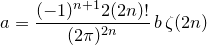
- A different approach (also described in this paper in Section 5) uses the tangent numbers again: Recall that the tangent numbers can, by definition, be read off from the Taylor series expansion of tan(x). If we are interested in the Tangent numbers T0…Tm, we can simply define T'n = (2m+1)! / (2n+1)! Tn, which are the coefficients of the Taylor expansion of (2m+1)tan(x) and, crucially, also integers. We can then approximate (2n+1)tan(10-p) for some sufficiently large p and read off the Tn! For instance, for m = 3 and p = 4, we get (2n+1)tan(10-p) = 0.5040 0000 1680 0000 0672 0000 0272, from which we can read off the values 5040, 1680, 672, 272. Converting these T'n back to Tn, we get 1, 2, 16, 272 as expected. With some tricks, all of this can be implemented entirely with integer arithmetic (of course, using powers of two instead of powers of ten); however, it is quite difficult to implement this efficiently because the numbers involved get absolutely huge – we're talking many millions of digits. The MC included a draft of an implementation of this as MC (power series), and it did okay.
- Our tutor Herr Großer went a bit overboard and implemented Harvey's multimodular algorithm that computes Bn modulo many different prime numbers (the MC is not quite sure how) and then uses the Chinese Remainder Theorem to reconstruct the actual value of Bn. This is probably the fastest known algorithm to date for large n, so it is not too surprising that Herr Großer's solution wins over the MC Sr's for n = 10000.
What have we learned this week?
- Exponential algorithms are not good, but not handing in a solution at all is much worse.
- Memoisation is a nice and straightforward way to gain performance.
- Doing a bit of research (e.g. googling) is good and can secure you a top place – but do not simply copy-paste code or you will make the MC grumpy. You do not want the MC to be grumpy. That goes for all the MCs you will encounter, but the MC Sr is the oldest and therefore already has a high baseline value of grumpiness.
- It is not quite obvious how to optimise in Haskell. The lecture will briefly talk about this, but probably not go into too much detail. As a quick primer:
- Haskell is lazy (if code doesn't get executed, it probably doesn't incur any cost, so eliminating it doesn't give you any benefit)
- However, large unevaluated thunks are usually bad because they consume a lot of memory, and a lot of memory means a lot of garbage collection.
- GHC is really good at optimising, so many ‘optimisations’ a beginner may try to do by hand will have next to no effect. In particular, operations on lists (map, filter, foldr, length, etc.) are usually fused, so attempting to pack all of that into a single tail-recursive function to avoid building the intermediate lists is commendable, but usually pointless.
- Efficient algorithms do not have to be long or ugly, especially in Haskell.
- Herr Großer has too much time on his hands.
By the way, the MC Sr is introducing a new feature next week: If you have any important comments for the MCs (e.g. an alternative solution that somehow does not make it through the test system), please include them in your submission like this to ensure they do not miss them:
{-MCCOMMENT
Hello MC! Here is my alternative solution:

bernoulli n = 4
-}
Die Ergebnisse der vierten Woche
| Top 30 der Woche | |||
|---|---|---|---|
| Platz | Wettbewerber*in | Performance | Punkte |
| 1. | Simon Stieger | 2.10 | 30 |
| 2. | Anton Baumann | 2.9 | 29 |
| 3. | Marco Haucke | 2.8 | 28 |
| 4. | Martin Fink | 2.7 | 27 |
| 5. | Bilel Ghorbel | 2.6 | 26 |
| 6. | Almo Sutedjo | 2.5 | 25 |
| 7. | Tobias Hanl | 2.4 | 24 |
| 8. | Maisa Ben Salah | 2.3 | 23 |
| 9. | Nikolaos Sotirakis | 2.2 | 22 |
| 10. | Leon Julius Zamel | 2.1 | 21 |
| 11. | Yi He | 2.0 | 20 |
| Jonas Maximilian Weigand | 2.0 | 20 | |
| Nico Greger | 2.0 | 20 | |
| 14. | Daniel Strauß | 1.0 | 10 |
| Johannes Bernhard Neubrand | 1.0 | 10 | |
| Christoph Wen | 1.0 | 10 | |
| Damian Depaoli | 1.0 | 10 | |
| Justus Schönborn | 1.0 | 10 | |
| Paul Andrei Sava | 1.0 | 10 | |
| Qingyu Li | 1.0 | 10 | |
| Jonas Fill | 1.0 | 10 | |
| Björn Henrichsen | 1.0 | 10 | |
| Dominik Glöß | 1.0 | 10 | |
| Steven Lehmann | 1.0 | 10 | |
| Xianer Chen | 1.0 | 10 | |
| Timur Eke | 1.0 | 10 | |
| Anna Franziska Horne | 1.0 | 10 | |
| Kevin Schneider | 1.0 | 10 | |
| Denis Belendir | 1.0 | 10 | |
| Margaryta Olenchuk | 1.0 | 10 | |
This week, we received an encouraging 96 (correct) submissions, teaching us to always award a homework point for the Wettbewerbsaufgabe. To whittle these down to a Top 30, we spell checked 5 misspelled words of 5-10 characters against a dictionary of the 100 most common english words. Even unoptimised solutions should be able to do this in a fraction of a second. Setting the cutoff at 2 s leaves us with 30 submissions. As usual, we also have some entries hors compétition: A hyperoptimized solution by the MC Sr, an implementation based on BK-trees by co-MC Rädle (the MC Jr Sr?), and one using a simple but highly effective optimization by co-MC Stevens (the MC Jr Jr). More on these later.
Similar to last week, we will proceed in stages to distinguish submissions with different asymptotic running times. In the first phase, we simply ran the same test as before but increased the size of the dictionary to 1000 words:
| Performance evaluation: 5 misspellings, dictionary size 1000 | ||
|---|---|---|
| Name | Time | |
| MC Sr | 0.03 s | |
| Simon Stieger | 0.03 s | |
| Anton Baumann | 0.03 s | |
| Marco Haucke | 0.04 s | |
| Bilel Ghorbel | 0.04 s | |
| Nikolaos Sotirakis | 0.04 s | |
| Tobias Hanl | 0.04 s | |
| Maisa Ben Salah | 0.05 s | |
| Almo Sutedjo | 0.05 s | |
| Leon Julius Zamel | 0.05 s | |
| Martin Fink | 0.06 s | |
| BK Tree (co-MC Rädle) | 0.06 s | |
| Yi He | 0.09 s | |
| Early Exit (co-MC Stevens) | 0.11 s | |
| Jonas Maximilian Weigand | 0.19 s | |
| Nico Greger | 0.23 s | |
| Daniel Strauß | > 5 s | |
| Johannes Bernhard Neubrand | > 5 s | |
| Christoph Wen | > 5 s | |
| Damian Depaoli | > 5 s | |
| Justus Schönborn | > 5 s | |
| Paul Andrei Sava | > 5 s | |
| Qingyu Li | > 5 s | |
| Jonas Fill | > 5 s | |
| Björn Henrichsen | > 5 s | |
| Dominik Glöß | > 5 s | |
| Steven Lehmann | > 5 s | |
| Xianer Chen | > 5 s | |
| Timur Eke | > 5 s | |
| Anna Franziska Horne | > 5 s | |
| Kevin Schneider | > 5 s | |
| Denis Belendir | > 5 s | |
| Margaryta Olenchuk | > 5 s | |
Despite the generous time limit of 5 s, this already eliminates a whopping 17 contestants. All of them implemented lightly optimized versions of the recurrence on the problem sheet, which leads to a comfortably exponential running time. Here is a relatively clean example of such a solution, using only material that has been covered in the lecture:
editDistance :: Eq a => [a] -> [a] -> Int
editDistance a b = dab (length a - 1) (length b - 1)
  where
    m = (length a) + (length b)
    dab i j = minimum [if i < 0 && j < 0 then 0 else m,
                       if i >= 0 then 1 + dab (i-1) j else m,
                       if j >= 0 then 1 + dab i (j-1) else m,
                       if i >= 0 && j >= 0 && a!!i == b!!j then dab (i-1) (j-1) else m,
                       if i >= 0 && j >= 0 && a!!i /= b!!j then 1 + dab (i-1) (j-1) else m,
                       if i >= 1 && j >= 1 && a!!i == b!!(j-1) && a!!(i-1) == b!!j then 1 + dab (i-2) (j-2) else m
                      ]

spellCorrect :: [String] -> [String] -> [[String]]
spellCorrect d [] = []
spellCorrect d (x:xs) = spellCorrectWord d x : spellCorrect d xs

spellCorrectWord :: [String] -> String -> [String]
spellCorrectWord d s =
  let dists = map (\ s' -> (s',editDistance s s')) d
      minDist = minimum (map snd dists)
  in map fst $ filter (\ (_,d) -> d == minDist) dists
There are two obvious approaches to improving the performance of spellCorrect: Make editDistance faster; or avoid running editDistance for every word in the dictionary. A good example of the latter approach can be found in Martin Fink's submission. While iterating through the dictionary, his correct function keeps track of the lowest edit distance found so far. If the difference in lengths between the search word and the next dictionary word is larger than this distance, then there is no need to compute the edit distance for this pair, since abs (length x - length y) is a lower bound on editDistance x y.
Co-MC Stevens takes this approach to the extreme. He passes the minimum distance found so far to his editDistance function, and simply aborts the computation of the distance if it can no longer be below this threshold. As we shall see, this is highly effective if there are words with low edit distance to the search string in the dictionary; which you would expect to be the case in a realistic spell checking scenario.
These optimizations do not improve the asymptotic worst case running time of the algorithm, however. In order to achieve a polynomial running time, all solutions that survived this round employ dynamic programming. That is, they avoid recomputing distances by storing intermediate values in lists or arrays. A somewhat readable example of this approach comes courtesy of Herr Zamel:
editDistance :: Eq a => [a] -> [a] -> Int
editDistance xs ys = mem !! (length xs) !! (length ys)
    where
        mem = [[ed (i,j) | j <- [0..(length ys)]] | i <- [0..(length xs)]]
        ed (i,j) = minimum $ filter (>=0) [c1 i j, c2 i j, c3 i j, c4 i j, c5 i j]
        c1 i j = if i == 0 && j == 0 then 0 else -1
        c2 i j = if i > 0 then (mem !! (i-1) !! j) + 1 else -1
        c3 i j = if j > 0 then (mem !! i !! (j-1)) + 1 else -1
        c4 i j = if i > 0 && j > 0 then if xs !! (i-1) == ys !! (j-1) then (mem !! (i-1) !! (j-1)) else (mem !! (i-1) !! (j-1)) + 1 else -1
        c5 i j = if i > 1 && j > 1 && xs !! (i-1) == ys !! (j-2) && xs !! (i-2) == ys !! (j-1) then (mem !! (i-2) !! (j-2)) + 1 else -1
Here, the results of individual calls to ed are stored in the table mem. This requires very little extra implementation effort compared to the naive solution but brings with it a huge improvement in performance.
For the next stage we move to a different corpus, containing misspellings made by British and American students. As a first test, we picked 100 misspellings at random and ran them against the entire dictionary of 6137 correctly spelled words:
| Performance evaluation: 100 misspellings, dictionary size 6137 | ||
|---|---|---|
| Name | Time | |
| MC Sr | 1.44 s | |
| Simon Stieger | 1.84 s | |
| Anton Baumann | 2.19 s | |
| Early Exit (co-MC Stevens) | 2.23 s | |
| BK-tree (co-MC Rädle) | 2.44 s | |
| Marco Haucke | 3.80 s | |
| Nikolaos Sotirakis | 4.75 s | |
| Bilel Ghorbel | 4.95 s | |
| Tobias Hanl | 5.13 s | |
| Almo Sutedjo | 5.33 s | |
| Maisa Ben Salah | 5.44 s | |
| Martin Fink | 6.36 s | |
| Leon Julius Zamel | 6.61 s | |
| Yi He | > 10 s | |
| Jonas Maximilian Weigand | > 10 s | |
| Nico Greger | > 10 s | |
The time limit of 10 s eliminates 3 further students, leaving us with a Top 10. The eliminated students implemented dynamic programming but construct and update their tables in very inefficient ways, mainly by using excessive amounts of ++ operations, which are linear in their first argument.
In order to get some separation between the remaining submissions, we increase the number of misspellings to 3000:
| Performance evaluation: 3000 misspellings, dictionary size 6137 | ||
|---|---|---|
| Name | Time | |
| MC Sr | 26.72 s | |
| Simon Stieger | 32.99 s | |
| BK-tree (co-MC Rädle) | 36.38 s | |
| Anton Baumann | 41.29 s | |
| Early Exit (co-MC Stevens) | 41.83 s | |
| Marco Haucke | 91.67 s | |
| Bilel Ghorbel | 104.79 s | |
| Nikolaos Sotirakis | 116.16 s | |
| Martin Fink | 121.47 s | |
| Maisa Ben Salah | 123.43 s | |
| Tobias Hanl | 125.93 s | |
| Almo Sutedjo | 130.01 s | |
| Leon Julius Zamel | 151.81 s | |
Co-MC Stevens' submission is still up there, even though it uses a completely unmemoized implementation of the edit distance. This is because the words in this dictionary are quite short, and it is therefore likely that a pair with low edit distance will be found relatively quickly. Once such a pair has been found, his early exit optimization is able to discard most words after looking at a few letters.
This drastically changes, however, once we begin to look at longer words where a pair with low edit distance may not be found easily. In order to find a suitable test case that shows this, English is no longer sufficiently powerful. Only by switching to good old Deutsch can we make use of words like Straßenentwässerungsinvestitionskostenschuldendienstumlage or Rinderkennzeichnungsfleischetikettierungsüberwachungsaufgabenübertragungsgesetz.
For our last test case, we used a dictionary derived from the duden corpus, but discarded all those boring words of fewer than 15 characters. This leaves us with 94061 words, which we tested against 20 Bandwurmwörter of 32 - 81 characters. This might seem pretty brutal, but some submissions were able to handle this test quite well:
| Performance evaluation: 20 Bandwurmwörter, dictionary size 94061 | ||
|---|---|---|
| Name | Time | |
| MC Sr | 16.81 s | |
| Simon Stieger | 21.90 s | |
| Anton Baumann | 22.18 s | |
| Martin Fink | 112.68 s | |
| BK-tree (co-MC Rädle) | 133.04 s | |
| Marco Haucke | 203.91 s | |
| Almo Sutedjo | 218.58 s | |
| Tobias Hanl | 294.11 s | |
| Bilel Ghorbel | 309.47 s | |
| Maisa Ben Salah | 355.84 s | |
| Leon Julius Zamel | 365.17 s | |
| Nikolaos Sotirakis | 583.92 s | |
| Early Exit (co-MC Stevens) | > 600 s | |
Notably, the Herren Stieger and Baumann were able to stay quite close to the MC Sr's contribution. Both implemented dynamic programming using arrays and added the previously described optimization that avoids computing the edit distance of pairs whose length differential is sufficiently large. Herr Fink also uses this optimization, but his choice of lists instead of arrays slows him down somewhat. Herr Stieger additionally implemented the early exit optimization.
To get a little bit of extra performance, the MC Sr strips common prefixes and suffixes before computing the edit distance and uses linear space in his editDistance implementation by keeping only two rows of the table. He also implemented parallelism, but our tests were run on a single thread. Otherwise, his solution is quite similar to Herr Stieger's.
Another avenue for optimization is preprocessing the dictionary, although none of the student submissions took this opportunity. Co-MC Rädle, however, stores his dictionary as a BK-tree, which is a tree where the edit distance between a node and its k-th child (if it exists) is exactly k. When running a search word against this tree representation of the dictionary, one uses the fact that the edit distance is a metric and thus fulfills the triangle inequality. We can search for words with distance of at most d from the search word as follows: If the distance between the root and the search word is n, then by the triangle equality, the distance between the k-th child and the search words is at least n-k. We therefore consider only children in the range [d-n..d+n] in our search, because children outside this range have a distance of at least n-(d+n+1) = d+1 to the search word.
This means that we do not need to compare every word in the dictionary against the search word; empirical results suggest that on an average search ~20% of the dictionary is considered. If a word is a possible candidate, however, the edit distance needs to be computed in full in order to determine which children need to be included in the search; no early exit optimization is possible. Additionally, we cannot discard words based on their length, because it is not sufficient to know that the edit distance is larger than a certain value -- we need to know the exact edit distance to proceed. This is why the BK-tree based implementation does well in the benchmarks, but is not able to compete with the very best solutions.
What have we learned this week?
- We should always award homework points for the Wettbewerbsaufgabe, lest we get fewer and fewer submissions.
- Wettbewerbspunkte need not be hard to come by; lightly optimized solutions scored 10 points this week.
- Dynamic programming can be simple to implement and highly effective.
- Computing something quickly is still slower than not computing it at all. (cf. co-MC Stevens)
- Sometimes different types of optimization can get in the way of each other, as is the case with BK-trees.
- The students are coming closer than ever to besting the venerable MC Sr.
Die Ergebnisse der fünften Woche
*cough cough, sniff, inhale* yes, this is the MC Jr speaking. Little did he know when leaving his beautiful office that he shall not return for a 3 days. The reason for his long absence are the long paths through the intriguing nature surrounding the Garchosibirsk campus that the 67 delightful submissions for week 5 were computing. The MC Jr owes you a great debt of gratitude for this splendid experience.
Moreover, he received obligatory, highly optimised, linear time submissions by the MC Sr and the tutor that has too much time on his hands: Herr Großer.
As a matter of fact, the longest path problem is quite computationally expensive (NP-hard) in general, but for DAGs, like the Garchosibirsk campus, the problem is rather easy to solve (linear time).
Just like his more senior fellow, the MC Jr decided to conduct several phases of elimination.
So let's get down to business to defeat the Huns 🎶 to trenn die Spreu vom Weizen 🌾.
The first pre-processing step, round -1 (minus one), consists of eliminating all submissions that do not pass the tests on the server.
At this phase, we already have to say goodbye to one of the top ranked participants, Herr Stieger, who did not submit a working solution.
Just by chance, the MC Jr actually discovered that Herr Stieger submitted a solution using the {-MCCOMMENT...-} feature, but
nevertheless, the provided solution uses the unsafe Data.Array.ST module that does not compile on the server.
We are sorry Herr Stieger, but same rules for everyone:
- The submission needs to pass the tests on the server
- An optional, alternative solution provided in the comments needs to at least compile on the server
Herr Stieger, by the way, used the topological order of the graph – an approach that many top-ranking FPETs fancied as we will see later on.
Edit 26.12.2019: After having a talk with the MC Sr, it was decided to change Herr Stieger's submission to use the safe Data.Array.ST.Safe import and make his submission part of the competition. The ranking was updated accordingly.
In round 0, the MC Jr decided to perform a very basic sanity check by running all submissions against the graph provided on the homework sheet:
Seeing all the tests pass made the MC Jr happier than a box of chocolate. But then, out of nowhere, the scary word appears: FAIL.
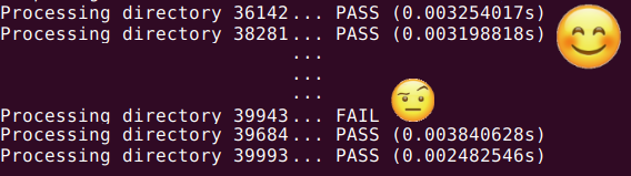
With great horror, he realised that one of his FPETs (Functional Programmers of Excellence in Training) failed the most simple test but still passed the tests on the submission server! He decided to have a look at the solution provided by the lucky Oleksandr Golovnya:
longestPath g t = head [snd x | x <- topsort [(v,0)| v <- fst g] (snd g), fst x == t]

topsort [] e = []
topsort (v:vs) e = [v] ++ topsort [(fst x, if elem (fst v,fst x) e && 1+snd v > snd x then 1 + snd v else snd x) | x <- vs] e
First things first: Let's clean up the code.
longestPath (vs,es) t = let ts = topsort [(v,0) | v <- vs] es in
   head [c | (t',c) <- ts, t' == t]

topsort [] es = []
topsort ((s,c):vs) es = (s,c) : topsort [(s, if elem (s,t) es then maximum (1 + c, c') else c') | (t,c') <- vs] es
That's better. Here are a few things to keep in mind:
- Split long expressions into simpler subexpressions to increase readability (e.g. let
tsdenote the result of thetopSortcall) - Use pattern matching on tuples to avoid
fstandsndcalls - Do not write
[x] ++ xsto concatenate a single element to a list; just usex : xs
Anyway, putting all the stylistic things aside, the topsort function sadly does not topologically order at all but merely recurses on all vertices in given order (which could be anything!) and updates the distances to all neighbours with higher index, completely neglecting the fact that there might be edges to vertices with a lower index.
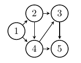
How this fails can easily be seen when we use Herr Golovnya's submission on our small example containing and edge from node 4 to 3:
longestPath = ([1..5] , [(1 ,2) ,(2 ,3) ,(2 ,4) ,(3 ,5) ,(1 ,4) ,(4 ,3) ,(4 ,5)]) 5 = 3
The MC Jr sadly made things too easy on the test server and only generated graphs not containing such edges. So, you got lucky this time and well-deserve your homework point Herr Golovnya, but you are sadly out of the competition. Remaining FPETs: 66 + 2
Next, the MC Jr started elimination round number 1: checking for cheeky FPETs that just assumed that the MC Jr's stroll will always start at vertex number 1.
Taking the following simple graph reveals the sloppy instruction readers:
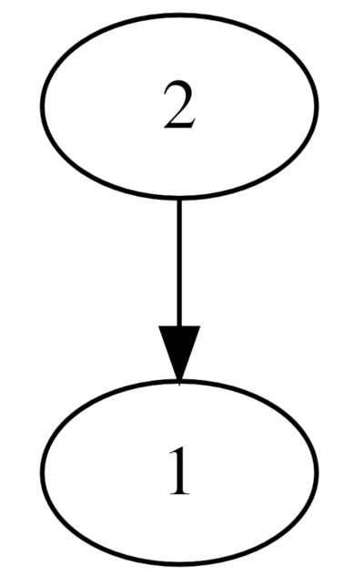
A long list of FAILs were printed on his GNU terminal of trust. 19 (that's almost a third of all submissions; #quickmaths) FPETs tried to trick the MC Jr.
Relentlessly, each and every one of them will be eliminated – the MC Jr will start his walks wherevere he wishes to!
Again, we have to say goodbye to some top-tier candidates at this stage, among others Frau Chernikova, Herr Soennecken, and Herr Haucke.
Just like Herr Stieger, they made use of a topological ordering algorithm.
The latter even hoped for some small-scale optimisations inlining his updateMap function and left the following comment:
Inlining this is akin to thinking that putting spoilers on your car adds horsepower, but now it looks a little more as if I knew what I was doing
{-# INLINE updateMap #-}

...
The MC Jr agrees and also suggests that instead of investing into small-scale optimisations, one should first prove one's implementaiton to be correct – in the best case, using Isabelle (#Dauerwerbesendung). Some other submissions got really confused with computer science and mathematical lingo, calling their topoligcal ordering a topology. The MC Jr hence kindly provides the following pictures that should clear up all confusion.

|

|
Finally, we get our hands feet dirty and start our first walk. A walk along 32 vertices. A walk so short, the MC Jr was barely able to leave the Magistrale.
A small number of 5 FPETs, however, took longer than a fifth of a second (an ETERNITY!) to compute the distance. Sad! Remaining FPETs: 42 + 2
And so the same game repeats: the MC Jr increases the number of nodes to 40 (a quick stroll to the Interimsgebäude), eliminating another 27 FPETs (15 + 2 remaining), and then, he cannot quite remember the exact number, but he guarantees something between 60 and 200 (a brisk walk to the U-Bahn), to eliminate a further 10 FPETs (5 + 2 remaining) that sadly did not quite make it into the group of big girls and boys.
Before continuing with the quarter-finals, the MC Jr decided to time the submissions kicked out thus far. After all, it is almost Christmas time and he wants to hand out some gifts aka. precious ranking points. Some rounds of competition on the Interimsgebäude graph led to the following ranking – congrats to all the winners so far 🎉:
| Result quarter-finalists | ||
|---|---|---|
| Rank | FPET | Points |
| 6. | Yi He | 25 |
| 7. | Mokhammad Naanaa | 24 |
| 8. | Matthias Ellerbeck | 23 |
| 9. | Emil Suleymanov | 22 |
| 10. | Pascal Ginter | 21 |
| 11. | Kaan Uctum | 20 |
| 12. | Sebastian Galindez Tapia | 19 |
| 13. | Tal Zwick | 18 |
| 14. | Tobias Hanl | 17 |
| 15. | Ricardo Vera Jacob | 16 |
| 16. | Yevgeniy Cherkashyn | 15 |
| 17. | Omar Eldeeb | 14 |
| 18. | Ernst Pappenheim | 13 |
| 19. | Leon Beckmann | 12 |
| 20. | Mira Trouvain | 11 |
| 21. | Erik Heger | 10 |
| 22. | Hui Cheng | 9 |
| 23. | Cosmin Aprodu | 8 |
| 24. | Björn Henrichsen | 7 |
| 25. | Daniel Anton Karl von Kirschten | 6 |
| 26. | Jonas Hübotter | 5 |
| 27. | Kevin Burton | 4 |
| 28. | Ali Mokni | 3 |
| 29. | Adrian Marquis | 2 |
| 30. | Heidi Albarazi | 1 |
Almost all quarter-finalists made use of basically the same idea: In order to compute the longest path from the source s to some node v, it suffices to recursively calculate the longest paths to v starting from v.
As, by assumption, our graph is a DAG and s is its only source node, the result of this computation will be the longest path from s to v.
In other words, if l(v) denotes the longest path from s to v, then l(v) satisfies the following recurrence relation:
l(v)=max({0} ∪ {l(w) | (w,v) ∈ E}).
This backwards traversal also has the nice effect that one does not need to explicitly search for the starting node s.
The MC Jr decided to show Herr Pappenheim's crisp one-line solution as a reference for this approach:
longestPath g@(vs, es) v = maximum (0:[1+(longestPath g x) | (x, a) <- es, a == v])
Note how Herr Pappenheim made use of the great as-patterns in order to inspect the components of g while still having the possibility to refer to g in its totality.
If the competition would have been about style and elegance, Herr Pappenheim surely would have won! ✨
Okay, now let's get real. For the semifinals, the MC Jr drew a graph from his office to the Maschinenwesen building. It's a dense graph containing 639 vertices, including the soft-opened Galileo (according to reliable sources, the hard opening is planned at about the same time as the opening of the BER). Running the semifinalist's submissions for one second reveals the four finalists. I am afraid, but the following FPETs got eliminated due to a timeout:
| Rank | FPET | Time | Points |
|---|---|---|---|
| 3. | Xiaolin Ma | 2.1s | 28 |
| 4. | Martin Achenbach | 6.22s | 27 |
| 5. | Le Quan Nguyen | TIMEOUT (>20s) | 26 |
An optimisation of the previously explained backwards traversal approach can be obtained by means of a tail-recursive implementation using an accumulator to store all so-far visited nodes and the so-far computed distance. This approach has been followed by Herr Nguyen, putting him on place 5 for this week. Congrats!
longestPath (node, edge) t = go [t] 0
 where go [] n = n-1
       go xs n = go (nub $ concat [ [w | (w,u)<-edge, u == x] | x<-xs]) (n+1)
Herr Ma and Herr Achenbach, however, made use of a topological order approach (that will be explained shortly), winning 28 and 27 points respectively. Congratulations! 🥳
For the finals, the MC Jr went to great pains and drew the whole Garchosibirsk campus containing a Fantastilliarde – in digits 20.000 – nodes and millions of edges using only a ruler and a compass. At first, he let the finalists compete on the whole dense graph he constructed. He then ran a second round on a very sparse graph that still contained 20.000 nodes but only 40.000 edges. The finalists' approaches can be summarised as follows:
- Herr MC Sr Manuel Eberl and Herr Ghorbel take the optimisation of the backwards traversal approach a step further. Herr Eberl uses an optimised version of
nubfor integers, hash maps instead of lists for quicker lookups, and a memoisation map storing the values of the so-far computed l(v) values. Herr Ghorbel decided to use Arrays and the graph library provided by Haskell instead.
Implementation by the MC Sr-- Faster O(n log n) nub specialised for integers. -- Probably doesn't make a difference but still. intNub :: [Int] -> [Int] intNub = map head . group . sort longestPath :: Graph -> Vertex -> Int longestPath (vs, es) v = longestPath' v where succMap = HS.map intNub $ HS.fromListWith (++) [(v, [u]) | (u, v) <- es] succs v = HS.lookupDefault [] v succMap m = HS.fromList [(v, longestPath'' v) | v <- vs] longestPath' v = fromJust (HS.lookup v m) longestPath'' v = maximum (0 : map ((+1) . longestPath') (succs v))
Implementation by Herr Ghorbel. It is not quite clear to the MC Jr whether using the topological sorting to construct the indices (maxi::[Int]->Int maxi [] = -1 maxi xs = maximum xs longestPath :: Graph-> Vertex -> Int longestPath (v,e) s = f s where cmp (a,_) (b,_) = compare a b min_v = minimum v max_v = maximum v graph = buildG (min_v,max_v) e tgraph = transposeG graph topo = topSort graph iTable = listArray (min_v,max_v) (map snd (sortBy cmp (zip topo [min_v..max_v]))) f x = 1 + maxi [memo!(iTable!nxt)|nxt<-(tgraph ! x)] memo = listArray (min_v,max_v) (map f topo)
iTable) for the memoisation mapmemohas any benefit. A quick experiment did not show any major performance difference when replacing the last four lines by the following two:
        f x = 1 + maxi [memo!nxt|nxt<-(tgraph ! x)]
        memo = listArray (min_v,max_v) (map f [min_v..max_v])
- Herr Großer and Herr Sutedjo used a varient of the following topological order approach:
- Create a topological order of the graph. This can be done, for example, by using a depth-first-search algorithm, or by using the following, more visually appealing, strategy: select all nodes without incoming edges, remove them from the graph (including their outgoing edges), and store them at the front of the ordering. Then repeat until you are left with nothing but cold void.
Topological order algorithm (source) - Process all vertices in topological order. For every vertex being processed, update the distances to its neighbours using the distance of the current vertex.
- Create a topological order of the graph. This can be done, for example, by using a depth-first-search algorithm, or by using the following, more visually appealing, strategy: select all nodes without incoming edges, remove them from the graph (including their outgoing edges), and store them at the front of the ordering. Then repeat until you are left with nothing but cold void.
It was a close race, but the final results are *can I please get some drums rolling*
🥁🥁🥁🥁🥁🥁🥁🥁🥁🥁🥁🥁🥁🥁🥁🥁🥁🥁🥁🥁🥁🥁🥁🥁🥁🥁🥁🥁🥁🥁🥁🥁🥁🥁🥁🥁🥁🥁🥁🥁🥁🥁🥁🥁🥁🥁🥁🥁🥁🥁🥁🥁🥁🥁🥁🥁🥁🥁🥁🥁🥁🥁🥁🥁🥁🥁🥁🥁🥁🥁🥁🥁🥁🥁🥁🥁🥁🥁🥁🥁🥁🥁🥁🥁🥁🥁🥁🥁🥁🥁🥁🥁🥁🥁🥁🥁🥁🥁🥁🥁🥁🥁🥁🥁🥁🥁🥁🥁| Results finalists | ||||
|---|---|---|---|---|
| Rank | FPET | Time dense graph | Time sparse graph | Points |
| 1. | Bilel Ghorbel | 3.65s | 0.47s | 30 |
| (out of competition) 2. | Markus Großer | 3.93s | 0.5s | |
| 3. | Almo Sutedjo | 3.99s | 0.52s | 29 |
| (out of competition) 4. | Herr MC Sr Manuel Eberl | 4.09s | 0.54s | |
Note: As you can clearly see in this beautifully formatted table, the MC Jr has a very strong web-development background.
So what have we learned this week?
- Make sure you submit something that passes the tests on the server.
- Passing the tests on the server does not guarantee correctness of the submission. Sorry Herr Golovnya and all "vertex number 1"-starters! But no need to worry. There's nothing lost and many points still to gain in upcoming competitions!
- Putting spoilers on one's car only gets you style points in Need for Speed but not the legendary FPV competition.
- A cow is a sphere. In symbols: 🐄 = 🌐
- Elegant and short implementations can get you very far
- Complicated implementations might get you even further *looking at Herr Großer*
- Using optimised libraries and cleverness gets you the furthest!
- Garchosibirsk is a mysterious, huge place.
- The MC Jr is a huge Mulan and Forrest Gump fan.
- Just to say it again: writing competition entries takes forever; it's 3am, good night! *drops mic*
Lastly, here's the combined result table for week 5. If you have any complaints, contact the MC Jr – he still is a MC in training and total correctness is hence not guaranteed.
Edit 26.12.2019: Herr Stieger's submission (modifed using safe array imports) has been added to the competition, scoring a bronze medal. Congratulations! The MC Jr decided to deduct 5 points for his unsafe imports that manually had to be changed and, as a matter of fairness, keep everyone else's points the same.
| Results week 5 | ||
|---|---|---|
| Rank | FPET | Points |
| 1. | Bilel Ghorbel | 30 |
| 2. | Almo Sutedjo | 29 |
| 2. | Simon Stieger | 28-5=23 |
| 3. | Xiaolin Ma | 28 |
| 4. | Martin Achenbach | 27 |
| 5. | Le Quan Nguyen | 26 |
| 6. | Yi He | 25 |
| 7. | Mokhammad Naanaa | 24 |
| 8. | Matthias Ellerbeck | 23 |
| 9. | Emil Suleymanov | 22 |
| 10. | Pascal Ginter | 21 |
| 11. | Kaan Uctum | 20 |
| 12. | Sebastian Galindez Tapia | 19 |
| 13. | Tal Zwick | 18 |
| 14. | Tobias Hanl | 17 |
| 15. | Ricardo Vera Jacob | 16 |
| 16. | Yevgeniy Cherkashyn | 15 |
| 17. | Omar Eldeeb | 14 |
| 18. | Ernst Pappenheim | 13 |
| 19. | Leon Beckmann | 12 |
| 20. | Mira Trouvain | 11 |
| 21. | Erik Heger | 10 |
| 22. | Hui Cheng | 9 |
| 23. | Cosmin Aprodu | 8 |
| 24. | Björn Henrichsen | 7 |
| 25. | Daniel Anton Karl von Kirschten | 6 |
| 26. | Jonas Hübotter | 5 |
| 27. | Kevin Burton | 4 |
| 28. | Ali Mokni | 3 |
| 29. | Adrian Marquis | 2 |
| 30. | Heidi Albarazi | 1 |
Die Ergebnisse der sechsten Woche
We at the Übungsleitung like to change things up and therefore the honourable task of writing this week's competition blog entry was bestowed upon the MC Jr Jr, Lukas Stevens.
In this week we received a grand total of 109 submissions that passed the tests on the server and had Wettbewerbstags.
As is tradition, some students managed to place the tags incorrectly which the MC Jr Jr generously fixed for them.
Additionally, the hacky lovingly handcrafted tool to evaluate the Wettbewerbseinreichungen is not nearly as sophisticated as the submission system; due to this Umstand, the tool breaks if a student omits the type annotations.
The MC Jr Jr embarked on a quest to fix these type annotations which was about as tedious as beating Pokémon without taking a single hit (this might be a slight hyperbole).
Tedium aside, the MC Jr Jr was delighted to see a new strategy emerge that allows students to eliminate other competitors.
This strategy, which we will discuss further down, forced one unlucky student to perform a Pofalla-Wende and thus we are left with 108 submissions.
Originally, this week's IBM Award for Software of Questionable Quality would have gone to a solution with 153 tokens; however, the MC Jr Jr noticed that the submission included the example prime program inside the tags upon closer inspection. This confirmed the suspicion that not even a very creative student could overcomplicate the task by that much. Instead, the award is granted to the solution of another student which is layed out in all its glory below.
t31 (a,b,c) = a
t32 (a,b,c) = b
t33 (a,b,c) = c

traceFractran :: [Rational] -> Integer -> [Integer]
traceFractran rs n
    | t31 aux2 = (t32 aux2) : (traceFractran rs (numerator $ t33 aux2))
    | otherwise = [n]
        where
            aux2 = aux rs n
            aux [] n = (False, 0, 0%1)
            aux (r:rs) n = if denominator (n%1 * r) == 1 then (True, n, n%1 * r) else aux rs n
Apparently, the student in question is not afraid of loosing a billion dollars and implements a tagged tuple that looks suspiciously like a null-reference (the first component being a flag that indicates whether the tuple is null).
This could be solved more elegantly using the Maybe type, but as Maybe hadn't been introduced in the lecture at that point the student may be forgiven in this instance.
Nevertheless, the model solution by the semi-venerable MC Jr Sr only uses material from the lecture while achieving a reasonable degree of conciseness.
With 49 tokens, this solution is only 2 tokens short of being in the top 30 and this without any serious effort to obfuscate optimise for number of tokens.
traceFractran fs n =
  let prods = [numerator (n%1 * f) | f <- fs, denominator (n%1 * f) == 1]
  in if null prods then [n] else n : traceFractran fs (head prods)
The following submission by Herr Tal Zwick illustrates that a few improvements to the model solution are sufficient to place in the top 30:
- Use
whereinstead oflet ... in. - The infix notation
`traceFractran`may allow you to omit parentheses. - In Haskell,
ifis an expression so it can be used (almost) anywhere.
Achieving rank 16 in the Wettbewerb doesn't require arcane Haskell knowledge after all!
traceFractran fs n = n:if null nfs then nfs else fs `traceFractran` head nfs
    where   ni = fromIntegral n
            nfs = [numerator $ f*ni | f <- fs, 1 == denominator (f*ni)]
Instead of optimising for tokens, Herr Andreas Resch unintentionally employed a novel technique to eliminate other competitors: Herr Resch notified the MC Jr Jr that his solution passes the testcases on the server despite being incorrect. Consequently, the MC Jr Jr came up with additional tests to determine which students tried to gain a competitive advantage through a disgraceful disregard for the specification. If not for those additional tests, the winner of this week's competition would have been Herr Peter Wegmann. He provided the following implementation with 29 tokens that is as elegant as it is wrong.
traceFractran xs y = y : concat [traceFractran xs $ numerator $ x * fromIntegral y | x<-xs, y `mod` denominator x == 0]
Here, traceFractran is called recursively every time the we get an integer as the product of a rational in the list xs and the accumulator y.
This gives erroneous results as soon we have more than one such product.
As Herr Resch was aware of this issue, he cleverly provided an alternative solution, which keeps him in the competition ganz im Gegenteil zu Herr Wegmann who is promptly eliminated.
The downside is that the alternative solution has 40 instead of the original 30 tokens which puts him in tenth place in the end.
The submission of one other competitor, namely Herr Emil Suleymanov, had the same bug.
Fortunately, his submission contained a simpler and also correcter version of traceFractran.
The MC Jr Jr has doubts that Herr Suleymanov knowingly circumvented the specification but he decided to let Gnade walten and keep him in the race with the latter version.
Nevertheless, this brings him from 29 up to 37 tokens thus placing him firmly on rank seven.
The takeaway is that this tactic should be applied judiciously lest you eliminate yourself from the top 30.
All of the above implementations are quite basic and only use material from the lecture.
Of course there are some people who just can't keep it simple like Herr Johannes Neubrand.
Not only does he use the constructor (:%), which not even a Sith would tell you about, to match on Rationals, he also just learnt about all kinds of monadic operators.
Such operators are used liberally throughout his implementation, sometimes even to the detriment of the token count (as seen in the implementation of integerProduct).
It shows that we teach him well because he is becoming a true Haskell programmer who values beauty over everything else.
The solution is actually (kind of) straightforward:
integerProductonly returns the result of the multiplication of its arguments if that result is an integer. Otherwise it returnsNothing.concatMap (traceFractran fs) rsconcatenates the lists that result from applyingtraceFractran fsto each element in rs.- Here,
msumreturns the first element in a list that isJust xandNothingotherwise. - Finally,
integerProduct n <$> fsis equivalent tomap (integerProduct n) fs.
integerProduct :: Integer -> Rational -> Maybe Integer
integerProduct x f = n <$ guard (d == 1)
    where n :% d = fromIntegral x * f

-- Alternative implementation of integerProduct by the MC Jr Jr
integerProduct x f = case fromIntegral x * f of
  n :% 1 -> Just n
  _ -> Nothing

traceFractran :: [Rational] -> Integer -> [Integer]
traceFractran fs n =
    n :                                 -- we were definitely able to reach this one
        ( concatMap (traceFractran fs)  -- because: instance Foldable (Maybe a)
        $ msum                          -- first Just or Nothing
        $ integerProduct n <$> fs
        )
Further interesting optimisation were done with monadic operators, e.g. Herr Haucke used mempty instead of [].
Nevertheless, to get near the top of the leaderboard, monadic operators were not necessary as the submissions of Herr Martin Fink and Herr Simon Stieger illustrate.
Both of them achieved rank 2 by essentially providing a correct version of Herr Wegmanns solution with 33 tokens.
The only significant adjustment is to use take 1 such that only the first product that results in an integer is considered in each step.
Thus, the code loses little of its elegance and still only uses material from the lecture.
traceFractran rs n = n : concat (take 1 [rs `traceFractran` floor (fromIntegral n * r) | r <- rs, n `mod` denominator r == 0])
With all that said, the best submission by Herr Almo Sutedjo did employ some monadic operators to get down to 30 tokens for which the MC Jr Jr sincerely congratulates him. This is an impressive feat considering that he not only surpassed all the other students but also bested Herr Markus Großer by 1 token whose resources don't seem to be infinite after all. The details of Herr Sutedjos solution are explained below.
- Again, the operator
<$>is used here instead ofmap. - The expression
liftM2 eqInteger truncate numeratorconstructs a function that compares the numerator of a rational numberrwith its truncated form (the integer closest torfrom 0). Thus, the expression returns true if, and only if,ris an integer. fromMaybeunwraps a Maybe and uses the first argument as a default value in case it encountersNothing.findtries to find an element in a list that satisfies the given predicate. This is also the function that Herr Oleksandr Golovnya was looking for. To find just the function you need, hoogle is a helpful tool.
traceFractran rs n = n : fromMaybe [] (traceFractran rs <$> numerator <$> (liftM2 eqInteger truncate numerator) `find` map (fromIntegral n *) rs)
Even though the above solution is impressive, there is still room for improvement: using mempty instead of [] and omitting the parentheses around liftM2 would have landed Herr Sutedjo at a comfortable 27 tokens.
This brings us very close to the ever-unbeatable MC Sr who came up with the following solution that has 26 tokens:
denominator &&& numerator <<< (* fromIntegral n)uses the combinators fromControl.Arrowto construct a function that first multiplies a rational numberrbynand then returns a tuple where the first component is denominator and the second component the numerator ofr * n.- After mapping this function over the list
xs, we find the first numerator whose corresponding denominator is 1 usinglookup 1. - Ultimately,
concatMap :: Foldable t => (a -> [b]) -> t a -> [b]is used to collect the results from the recursive calls into a list. Note that the we fold over the Maybes that are returned bylookup 1.
traceFractran xs n = n : traceFractran xs `concatMap` lookup 1 (map (denominator &&& numerator <<< (* fromIntegral n)) xs)
So what have we learned today?
- Until further notice, the MC Jr Jr kindly requests that the students annotate functions with their type within the WETT tags (type annotations are ignored when counting tokens).
- Short solution don't require material beyond that of the lecture.
- Using the MCCOMMENT tag, you may provide the MCs with pathological test cases to eliminate other competitors. But be careful not to eliminate yourself.
- Monadic operators are fun (at least to some people).
Lastly, we come to the the table of ultimate truth provided that the MC Jr Jr did not make any mistakes, which you should bring to his attention upon discovery.
| Die Ergebnisse von Woche 6 | |||
|---|---|---|---|
| Rank | Author | Tokens | Points |
| 1. | Almo Sutedjo | 30 | 30 |
| 2. | Martin Fink | 33 | 29 |
| Simon Stieger | 33 | ||
| 4. | Le Quan Nguyen | 35 | 27 |
| 5. | Marco Haucke | 36 | 26 |
| Yi He | 36 | ||
| 7. | Emil Suleymanov | 37 | 24 |
| 8. | Yannan Dou | 38 | 23 |
| 9. | Omar Eldeeb | 39 | 22 |
| 10. | Andreas Resch | 40 | 21 |
| 11. | Johannes Bernhard Neubrand | 41 | 20 |
| Xiaolin Ma | 41 | ||
| 13. | Ernst Pappenheim | 42 | 18 |
| Ujkan Sulejmani | 42 | ||
| Felix Trost | 42 | ||
| 16. | Tal Zwick | 43 | 15 |
| 17. | Jonas Jürß | 44 | 14 |
| David Maul | 44 | ||
| Yecine Megdiche | 44 | ||
| Kevin Schneider | 44 | ||
| Florian Melzig | 44 | ||
| 22. | Janluka Janelidze | 45 | 9 |
| Maisa Ben Salah | 45 | ||
| 24. | Tobias Hanl | 46 | 7 |
| Torben Soennecken | 46 | ||
| Kristina Magnussen | 46 | ||
| Steffen Deusch | 46 | ||
| Kevin Burton | 46 | ||
| 29. | Anna Franziska Horne | 47 | 2 |
| Chien-Hao Chiu | 47 | ||
Die Ergebnisse der siebten Woche
The MC Jr Sr was sorely disappointed to only receive 46 correct solutions this week. To make matters worse, some students are rather shy and omitted the WETT tags, leaving us with just 28 submissions. Passing up free Wettbewerbspunkte — in this economy? Maybe the students are getting weary after toiling in the Haskell mines for nigh on two months; maybe we should avoid arcana like transitive or closure in the problem statements. Anyhow, we shall have to make due with this meagre harvest.
This week's longest correct solution weighs in at a War and Peace-rivalling 356 tokens:
filterFor :: Eq a => [(Integer,(a,a))] -> [(Integer,(a,a))]
filterFor [] = []
filterFor ((xc, (x1, x2)):xs) = case find (\(yc, (y1, y2)) -> y1 == x1 && y2 == x2 && yc <= xc) xs of
  Just _  -> filterFor xs
  Nothing -> (xc, (x1, x2)):filterFor xs

comp :: Eq b => [(Integer,(a,b))] -> [(Integer,(b,c))] -> [(Integer,(a,c))]
comp [] _ = []
comp _ [] = []
comp xs ys = [(xn + yn, (fst xt, snd yt)) | (xn, xt) <- xs, (yn, yt) <- ys, snd xt == fst yt]

trancl :: Eq a => [(Integer,(a,a))] -> [(Integer,(a,a))]
trancl xs = (reverse
        . filterFor2
        . sortBy (\(x1, _) (x2, _) -> compare x2 x1))
        (multipleComp xs [] [])


filterFor2 :: Eq a => [(Integer,(a,a))] -> [(Integer,(a,a))]
filterFor2 [] = []
filterFor2 ((xc, (x1, x2)):xs) = case find (\(yc, (y1, y2)) -> y1 == x1 && y2 == x2 && yc <= xc) xs of
  Just _  -> filterFor xs
  Nothing -> (xc, (x1, x2)):filterFor xs

multipleComp :: Eq a => [(Integer,(a,a))] -> [(Integer,(a,a))] -> [(Integer,(a,a))] -> [(Integer,(a,a))]
multipleComp [] _ _ = []
multipleComp xs [] _ = multipleComp xs xs xs
multipleComp xs ys acc = let currComp = filterFor3 acc (comp ys xs) in
      if currComp == [] then acc else (multipleComp xs currComp (acc ++ currComp))

filterFor3 :: Eq a => [(Integer,(a,a))] -> [(Integer,(a,a))] -> [(Integer,(a,a))]
filterFor3 _ [] = []
filterFor3 [] ys = ys
filterFor3 xs ((yc, (y1, y2)):ys) = case find (\(xc, (x1, x2)) -> x1 == y1 && x2 == y2 && xc < yc) xs of
  Just _ -> filterFor3 xs ys
  Nothing -> (yc, (y1, y2)):filterFor3 xs ys
There is some obvious code duplication here (One filterFor really ought to be enough for anybody) but other than that this is quite reasonable. The input is composed with itself until no new elements are generated (multipleComp) and then filtered to include only shortest paths. The additional sorting and reversing of the output should be unnecessary. Even the shortest solutions follow this basic approach, but are not quite as frivolous in introducing auxiliary functions.
One step up in conciseness is this particularly readable solution due to Herr Trost:
minRelations :: Eq a => [(Integer, (a, a))] -> [(Integer, (a, a))]
minRelations xs = nubBy (\(n1, (a1, b1)) (n2, (a2, b2)) -> a1 == a2 && b1 == b2) (sortBy (\(n1, a1) (n2, a2) -> compare n1 n2) xs)


comp :: Eq b => [(Integer,(a,b))] -> [(Integer,(b,c))] -> [(Integer,(a,c))]
comp fs gs = [(n1 + n2, (fa, gc)) | (n1, (fa, fb)) <- fs, (n2, (gb, gc)) <- gs, fb == gb]


trancl :: Eq a => [(Integer,(a,a))] -> [(Integer,(a,a))]
trancl xs = tranclRec (minRelations xs)
    where
        tranclRec xs
            | minRelations (xs ++ comp xs xs) == xs = xs
            | otherwise = tranclRec (minRelations (xs ++ comp xs xs))
He avoids unneccessarily introducing multiple functions for composition and filtering. One area where this solution could be shortened and made more readable are the calls to nubBy and sortBy. Specifically, sortBy (\(n1, a1) (n2, a2) -> compare n1 n2 compares tuples by their first element. Luckily the combinator on from Data.Function facilitates just that. It is defined as (.*.) `on` f = \x y -> f x .*. f y, i.e. it applies a function f to both its arguments and then combines the results using the binary operator (.*.). In our case we want to apply fst to the tuples and the compare them, so the above expression can be written neatly as sortBy (compare `on` fst). To squeeze out an extra token we can write this as (comparing fst) using the comparing function from Data.Ord.
Similarly, nubBy (\(n1, (a1, b1)) (n2, (a2, b2)) -> a1 == a2 && b1 == b2) removes duplicates by comparing the second element of the input tuples for equality. This can be shortened to nubBy ((==) `on` snd).
This brings us to this week's winning solutions. We beginn with Herr Baumann, who wins a silver medal with the following 73 token solution, that manages to be concise and supremely readable:
trancl :: Eq a => [(Integer,(a,a))] -> [(Integer,(a,a))]
trancl r = if r == new
           then r
           else trancl new
  where
    new = nubBy ((==) `on` snd)
          $ sortBy (comparing fst)
          $ r ++ [(c1+c2, (a, d)) | (c1, (a, b)) <- r, (c2, (c, d)) <- r, b == c]
The basic approach here remains the same, but he gains some tokens by inlining comp and the sorting and filtering steps. He also uses the previously described combinators comparing and on. Herr Baumann comes very close to the MC Sr, who manages to shave off an additional 4 tokens with the following 69 token solution:
trancl :: Eq a => [(Integer,(a,a))] -> [(Integer,(a,a))]
trancl r = if r == r' then r else trancl r'
  where r' = nubBy ((==) `on` snd) . sortBy (comparing fst) $ r ++
             [(m + n, (fst x, snd y)) | (m, x) <- r, (n, y) <- r, snd x == fst y]
The only difference here is the slightly more token-efficient pattern matching on the tuples in the list comprehension. I does not end here however. For the first time this semester, a student has managed to outtoken the Master of Tokens himself. Herr Nguyen beats him by 3 tokens with one weird library function the MC does not want you to know about: sortOn. Okay, the function is not even that weird; sortOn f is simply equivalent to sortBy (comparing f). Here is Herr Nguyen's historic 66 token solution in its full glory:
trancl :: Eq a => [(Integer,(a,a))] -> [(Integer,(a,a))]
trancl xs= if findTrancl == xs then xs else trancl findTrancl
 where findTrancl = nubBy (on (==) snd) $sortOn fst  $xs++[(i+j,(fst ab, snd cd))|(i,ab)<-xs, (j,cd)<-xs,snd ab==fst cd]
Before we conclude this week's competition, an honourable mention. The MC Jr Sr intended the weights of the relation to be nonnegative, but did not specify this in the problem statement. Most students — in particular all of the solutions we have looked at in this post — implicitly made this assumption anyway, and enter infinite loops if there is a negative length cycle in the input. Not so Herr Janelidze. He followed the problem statement to a tee, implementing the Bellman-Ford algorithm to handle arbitrary relations. As a token (haha) of respect and a little Aufwandsentschädigung, the Übungsleitung awards him 5 bonus points.
So what have we learned today?
- At its best, Haskell can be concise and readable.
- The Übungsleitung should try to pick more interesting problems for the Wettbewerb, or at least couch them in more attractive language.
- Relatedly, the MC Jr Sr should work harder to write clear problem statements, lest he sends some poor students down a rabbit hole. (cf. Herr Janelidze)
- Knocking the MC Sr of his perch — high atop an ivory tower — may be more feasible than previously imagined.
Here then, are this weeks results. As always, alle Angaben ohne Gewähr; let us know if anything is amiss. Addenda: We incorrectly ruled out Almo Sutedjo's 96 token solution and Martin Fink's 100 token solution, they are retroactively awarded 24 points.
| Die Ergebnisse von Woche 7 | |||
|---|---|---|---|
| Rank | Author | Tokens | Points |
| 1. | Le Quan Nguyen | 66 | 30 |
| 2. | Anton Baumann | 73 | 29 |
| 3. | Yi He | 77 | 28 |
| 4. | Bilel Ghorbel | 82 | 27 |
| 5. | Simon Stieger | 89 | 26 |
| 6. | Yecine Megdiche | 90 | 25 |
| 7. | Almo Sutedjo | 96 | 24 |
| 7. | Martin Fink | 100 | 24 |
| 7. | Johannes Bernhard Neubrand | 101 | 24 |
| 8. | Tal Zwick | 106 | 23 |
| 9. | Marco Haucke | 107 | 22 |
| 10. | Felix Rinderer | 116 | 21 |
| 11. | Korbinian Stein | 127 | 20 |
| 12. | Kaan Uctum | 128 | 19 |
| 13. | Christo Wilken | 129 | 18 |
| 14. | Tung Nguyen | 134 | 17 |
| 15. | Stephan Baller | 136 | 16 |
| 16. | Tobias Hanl | 136 | 15 |
| 17. | Simon Hundsdorfer | 137 | 14 |
| 18. | Felix Trost | 137 | 13 |
| 19. | Ernst Pappenheim | 142 | 12 |
| 20. | Wen Qing Wei | 173 | 11 |
| 21. | Steffen Deusch | 177 | 10 |
| 22. | Hui Cheng | 204 | 9 |
| 23. | Janluka Janelidze | 220 | 8 + 5 |
| 24. | Johannes Schwenk | 234 | 7 |
| 25. | Joel Koch | 235 | 6 |
| 26. | Lukas Flesch | 328 | 5 |
| 27. | Zhiyi Pan | 343 | 4 |
| 28. | Anna Franziska Horne | 356 | 3 |
Die Ergebnisse der achten Woche
There were 167 solutions this week, ‘this week’ being ‘the week before Christmas, about 4 weeks ago’. Sorry about that, but even the MC Sr celebrates Christmas to some extent, and then someone invited him to give a talk in Pittsburgh in the first week of January, so he did not have much time for Wettbewerb matters.
Anyway, now he is back, so enjoy the account of a severely jetlagged MC ploughing through 167 correct student submissions. The largest one has 160 tokens:
shoefa [] = 0
shoefa xs = checkV [x|x<-xs, x/=0] 0 0
            where checkV [] v n = n
                  checkV xs 0 0 = if (head xs < 0) then (checkV (tail xs) (-1) (0)) else (checkV (tail xs) (1) (0))
                  checkV xs 1 n = if (head xs < 0) then (checkV (tail xs) (-1) (n+1)) else (checkV (tail xs) (1) (n))
                  checkV xs (-1) n = if (head xs < 0) then (checkV (tail xs) (-1) (n)) else (checkV (tail xs) (1) (n+1))
There is quite a lot of duplication of code in there, plus some unnecessary parentheses. The recursion would also be expressed more idiomatically using pattern matching instead of head and tail. The general idea behind this solution is, however, perfectly fine: remove all the zeros from the list and recurse through it left-to-right, remembering the last sign that we have seen and the total number of sign changes so far. However, the non-tail-recursive approach would likely be better for saving tokens (at the cost of performance).
A much more streamlined and non-tail-recursive version of this approach was done by Herr Mayr in 48 tokens:
shoefa xs = help clean (head clean) where clean = filter (/= 0) xs
help [] _ = 0
help (x:xs) last = if signum x /= signum last then 1 + help xs x else help xs last
Note that he cleverly defines the auxiliary function on the toplevel (not using let or where). This is not good style, but it saves him one token. However, three tiny modifications could have saved him another 4 tokens: replacing parentheses with $, reordering the two equations for help so that we can replace [] by the wildcard _, and factoring the common part out of the if:
shoefa xs = help clean $ head clean where clean = filter (/= 0) xs
help (x:xs) last = help xs x + if signum x /= signum last then 1 else 0
help _ _ = 0
However, even that would unfortunately have been nowhere near enough for the Top 30 this week, since competition was quite tough. Herr Schneider just missed the Top 30 with the following very clever 33-token solution, which is the shortest recursive one:
shoefa (x:y:xs) = fromEnum (x*y<0) + shoefa (y*2+signum x:xs)
shoefa _ = 0
He exploits two things here: first, that fromEnum False = 0 and fromEnum True = 1, and second that for integers a and b, the sign of 2b+a equals the sign of a if b = 0, and the sign of b otherwise. This allows him to skip zeros in the list implicitly, while most other solutions have to filter them out first. The non-tail-recursive recursion here will likely make this quite inefficient for long input lists (linear space requirement vs constant space), but we do not care about that this week. It is sad that Herr Schneider's ingenuity was not rewarded with any points – unfortunately, it seems that it was simply not possible to enter the Top 30 with a recursive solution.
So what did it take to get into the Top 30? Dinh Luc managed it with the following approach:
shoefa xs = length (filter (<0) (zipWith (*) cs  $ tail cs))
  where cs = filter (/=0) xs
The idea here is to kick out all the zeros, then pair up every number in the list with the one after it, and count the number of such pairs where the two numbers in it have different signs. Note that this version also has fairly okay performance A number of students have similar solutions, culminating in the following work of abstract art by Herr Neubrand, which consists of a mere 17 tokens (not a single one of which is a parenthesis!):
shoefa = filter toBool              -- remove zeroes
     >>> map signum
     >>> zipWith subtract <*> tail  -- transform to differences of signs    (equals -> 0)
     >>> filter toBool              -- keep only steps with differing signs (values /= 0)
     >>> length
What is going on here? Well, first of all, Herr Neubrand does not refer to any variables in his code; he describes the shoefa function entirely using combinators such as function composition. This can save tokens if used wisely, and the name for this technique is point-free style (clearly a misnomer: since function composition is usually written as ., it tends to contain a lot of points. And as you can see with this submission, it is also often rewarded with points in the Wettbewerb.
To unravel the mystery of Herr Neubrands solution, one needs to know the following things:
- The operator (>>>) is just the flipped version of the (.) operator you know from the lecture (f >>> g = g . f, or (f >>> g) x = g (f x)).
- When given an integer, the toBool function from the depths of Haskell's foreign function interface simply returns False if the integer is 0 and True otherwise, mirroring the way ancient languages like C treat integers in conditionals.
- (<*>) is another appearance of the reader monad, whose details shall remain in the dark. Let it just be said that (f <*> g) = \x -> f x (g x).
You may wonder why he chose to use (>>>) instead of (.). The reason is that unlike (.), (>>>) has a lower precedence than (<*>) and can therefore be used here without any parentheses.
The MCs' solutions and all of the top 20 solutions (other than Herr Neubrand's) use the following approach, e.g. Herr Khitrov with 19 tokens:
shoefa = max 0 . pred . length . group . map signum . filter (/= 0)
This approach uses the group function to partition the list into blocks of adjacent numbers having the same sign and then counts how many of these blocks there are: clearly, the number of sign changes is just that number minus one – except in the case of an empty list, in which case we would get -1 instead of 0, which is rectified by putting a max 0 in the front. The winning solutions by the Herren Haucke and Soennecken are virtually identical to the MCs' combined solution:
shoefa = length . drop 1 . group . map signum . filter toBool
The toBool instead of (/= 0) saves 3 tokens, and writing length . drop 1 instead of max 0 . pred . length saves another 2, which gets us from 19 to 14.
And that brings us to the results. What a delightfully competitive week! There are quite a lot of ties (especially for 4th place), which is why the MC decided to adjust the usual place-to-points scheme a little bit in order to avoid giving the ten people in place 4 almost as many points as the two in first place:
Lessons for this week:
- Duplication of code is usually bad.
- Haskell has good high-level combinators that can lead to code that is both shorter and more understandable.
- <*> in the reader monad is not one of them.
- Some students are really catching up with the MCs
- The MC saw quite a lot of unnecessary parenthesis in the code this week, including things like map (signum) xs. For operators like ++ and :, the precedence rules in Haskell are indeed not quite obvious and unnecessary parentheses are fine in those cases (at least outside the Wettbewerb). But in the absence of binary operators, there is really no excuse for them. The MC would therefore really like to encourage you to learn how function application works. Haskell is a functional language, so it's kind of an important concept. 😉
| Die Ergebnisse von Woche 8 | |||
|---|---|---|---|
| Rank | Author | Tokens | Points |
| 1. | Torben Soennecken | 14 | 30 |
| Marco Haucke | 14 | 30 | |
| 3. | Almo Sutedjo | 16 | 28 |
| 4. | Johannes Bernhard Neubrand | 17 | 23 |
| Konstantin Berghausen | 17 | 23 | |
| Rafiq Nasrallah | 17 | 23 | |
| Simon Stieger | 17 | 23 | |
| Yi He | 17 | 23 | |
| Alwin Stockinger | 17 | 23 | |
| Tal Zwick | 17 | 23 | |
| Daniel Petri Rocha | 17 | 23 | |
| Lukas Metten | 17 | 23 | |
| Jonas Lang | 17 | 23 | |
| 14. | Mira Trouvain | 19 | 15 |
| Ilia Khitrov | 19 | 15 | |
| Jonas Jürß | 19 | 15 | |
| Omar Eldeeb | 19 | 15 | |
| Martin Fink | 19 | 15 | |
| 19. | Janluka Janelidze | 24 | 12 |
| Mokhammad Naanaa | 24 | 12 | |
| Bastian Grebmeier | 24 | 12 | |
| 22. | Anton Baumann | 25 | 8 |
| Simon Hundsdorfer | 25 | 8 | |
| Oleksandr Golovnya | 25 | 8 | |
| 25. | Felix Trost | 26 | 6 |
| 26. | Christoph Reile | 27 | 5 |
| 27. | Dinh Luc | 30 | 3 |
| Peter Wegmann | 30 | 3 | |
| Tobias Hanl | 30 | 3 | |
| 30. | Bilel Ghorbel | 31 | 1 |
| Felix Rinderer | 31 | 1 | |
Die Ergebnisse der neunten Woche
I doubt that anyone implemented a CDCL-solver.
This week's challenge ("efficient SAT-solving 101") left room for many different optimisations and an endless amount of time could be spent on tuning one's implementation to the extreme. And without a doubt: our excellent students did indeed surpass the expectations.
For the evaluation, the MC Jr decided to run all submissions against 9 different test-suites and measure the performance. Most of the test-suites have already been mentioned on the exercise sheet, but also a few new ones have been added. Let's see who is going to win the prestigous SAT-championship of 2020 🏆!
Test 0: The Simplifier
As a warm-up test, the MC Jr measured the performance of the submissions' simplifier (simpConj on the exercise sheet).
However, nothing exciting happened at this point and all submissions performed almost equally well.
Test 1: Positive Literals
The first test-suite consisted of instances where each clause Ci contained at least one positive literal Li.
Such instances are always trivially satisfiable: set the variable of each Li to True and all remaining variables to arbitrary values.
The MC Jr generated 3 instances using the following parameters:
| Instance | Number of clauses | Number of variables | Max clause size | Frequency of positive variables | Frequency of negative variables |
|---|---|---|---|---|---|
| 1 | 446 | 10 | 10 | 1 | 1 |
| 2 | 21865 | 50 | 30 | 1 | 1 |
| 3 | 126870 | 60 | 50 | 1 | 1 |
Although it was stated on the exercise sheet, no student explicitly implemented any optimisations for this case.
Nevertheless, 30 out of 35 submissions still made it in the given timeframe of 40 seconds.
Some submissions were even very close to being on a par with the MC Jr, whose submission contained a special optimisation for these kind of formulas.
How come you might wonder?
Well, many students decided to simply pick the first unassigned variable in each round and assign it to True.
This works pretty well in this case of course, but will fail horribly in the next test-suite...
| Results test-suite 1: positive literals | ||
|---|---|---|
| Rank | Name | Time (seconds) |
| 1 | MC Jr | 26.276429 |
| 2 | Martin Habfast | 26.501732 |
| 3 | Johannes Bernhard Neubrand | 27.09761 |
| 4 | Haoyang Sun | 27.115166 |
| 5 | Daniel Strauß | 27.314486 |
| 6 | Steffen Deusch | 27.686936 |
| 7 | Marco Haucke | 27.811313 |
| 8 | Mokhammad Naanaa | 27.834761 |
| 9 | Torben Soennecken | 28.102151 |
| 10 | Peter Wegmann | 28.132764 |
| 11 | Kevin Schneider | 28.226784 |
| 12 | Nico Greger | 28.411079 |
| 13 | Aria Talebizadeh-Dashtestani | 28.571546 |
| 14 | Stephan Schmiedmayer | 28.613498 |
| 15 | Simon Stieger | 29.712261 |
| 16 | Dominik Schuler | 29.712261 |
| 17 | Christian Brechenmacher | 29.874143 |
| 18 | Konstantin Berghausen | 29.920745 |
| 19 | Jonas Lang | 29.940286 |
| 20 | Leon Blumenthal | 30.194362 |
| 21 | Leon Beckmann | 30.684815 |
| 22 | Daniel Anton Karl von Kirschten | 30.885557 |
| 23 | Tobias Jungmann | 31.428779 |
| 24 | Janluka Janelidze | 31.685789 |
| 25 | Kseniia Chernikova | 31.821769 |
| 26 | Felix Trost | 31.91729 |
| 27 | Tal Zwick | 32.797127 |
| 28 | Almo Sutedjo | 34.394997 |
| 29 | Martin Fink | 36.710968 |
| 30 | Boning Li | 38.764843 |
Test 2: Negative Literals
Test-suite numéro deux is the dual of numéro uno: each clause Ci contained at least one negative literal Li.
Hence, we can simply set the variable of each Li to False and all remaining variables to arbitrary values.
The MC Jr generated 3 instances using the following parameters:
| Instance | Number of clauses | Number of variables | Max clause size | Frequency of positive variables | Frequency of negative variables |
|---|---|---|---|---|---|
| 1 | 173 | 10 | 10 | 1 | 1 |
| 2 | 32445 | 50 | 30 | 1 | 1 |
| 3 | 110643 | 50 | 60 | 1 | 1 |
Again, the MC Jr granted each solver 40 seconds of his precious laptop computing power.
While this time submissions that carelessly tried to set each variable to True got punished, efficient implementations
– though not having any special case optimisation for this test-suite –
climbed up the ladder, being almost equally fast as the MC Jr's special case optimisation.
We shall see in the upcoming test-suites what kind of optimisations these students applied.
But first, here is the ranking for test-suite 2:
| Results test-suite 2: negative literals | ||
|---|---|---|
| Rank | Name | Time (seconds) |
| 1 | MC Jr | 24.480299 |
| 2 | Daniel Strauß | 24.855054 |
| 3 | Marco Haucke | 25.729774 |
| 4 | Kevin Schneider | 25.947265 |
| 5 | Mokhammad Naanaa | 25.947316 |
| 6 | Peter Wegmann | 26.134727 |
| 7 | Torben Soennecken | 26.38508 |
| 8 | Johannes Bernhard Neubrand | 26.535151 |
| 9 | Nico Greger | 26.783645 |
| 10 | Simon Stieger | 27.502702 |
| 11 | Dominik Schuler | 27.763788 |
| 12 | Daniel Anton Karl von Kirschten | 28.356478 |
| 13 | Janluka Janelidze | 28.955485 |
| 14 | Leon Beckmann | 28.985623 |
| 15 | Jonas Lang | 29.200797 |
| 16 | Konstantin Berghausen | 29.55542 |
| 17 | Leon Blumenthal | 29.757887 |
| 18 | Steffen Deusch | 29.974094 |
| 19 | Aria Talebizadeh-Dashtestani | 30.030047 |
| 20 | Boning Li | 30.105783 |
| 21 | Kseniia Chernikova | 30.106472 |
| 22 | Stephan Schmiedmayer | 30.187932 |
| 23 | Martin Habfast | 30.549589 |
| 24 | Haoyang Sun | 30.786313 |
| 25 | Tobias Jungmann | 30.874324 |
| 26 | Felix Trost | 31.136271 |
| 27 | Almo Sutedjo | 31.777069 |
| 28 | Martin Fink | 34.229154 |
| 29 | Tal Zwick | 37.148001 |
Test 3: Pure Literals
For the third test-suite, the MC Jr checked whether his brave students paid attention in their discrete structures classes:
the pure literal rule, as you all should remember, says that if some variable v occurs strictly positively or negatively, then it is safe to set
v to True or False, respectively.
To generate the problem set, the MC Jr introduced two new variables: bn and bp. Each variable of index ≤ bn will be generated strictly negatively and each variable of index ≥ bp will be generated strictly positively. Variables between bn and bp will be generated according to the passed frequency of negative and positive variables. The following parameters were used to create 6 instances:
| Instance | Satisfiable | Number of clauses | Number of variables | Max clause size | Frequency of positive variables | Frequency of negative variables | bn | bp |
|---|---|---|---|---|---|---|---|---|
| 1 | True | 100 | 10 | 10 | 1 | 1 | 3 | 8 |
| 2 | False | 3000 | 30 | 15 | 1 | 1 | 12 | 18 |
| 3 | False | 10000 | 50 | 40 | 1 | 1 | 21 | 27 |
| 4 | True | 50000 | 100 | 40 | 1 | 1 | 50 | 51 |
| 5 | False | 80000 | 100 | 40 | 1 | 1 | 48 | 51 |
| 6 | True | 120000 | 1000 | 50 | 1 | 1 | 500 | 501 |
45 seconds, the MC Jr decided, shall suffice for all 6 instances... but only 4 tough submissions made it in time. Congrats to Herr Megdiche at this point who left his competitors far behind.
| Results 1 test-suite 3: pure literals | ||
|---|---|---|
| Rank | Name | Time (seconds) |
| 1 | Yecine Megdiche | 33.634559 |
| 2 | MC Jr | 39.547038 |
| 3 | Kevin Schneider | 40.619992 |
| 4 | Martin Fink | 43.37776 |
So did only 3 students pay attention in their discrete structures classes? Of course not! To the MC Jr's great delight, he saw that many more students did indeed remember what they were taught in year one at TUM. And since the MC Jr has a good heart – he hopes you agree ❤️ – submissions that solved 5 out of 6 problems in time shall be ranked in a separate list:
| Results 2 test-suite 3: pure literals | ||
|---|---|---|
| Rank | Name | Time up to instance 5 (seconds) |
| 5 | Christian Brechenmacher | 15.144 |
| 6 | Almo Sutedjo | 16.196322 |
| 7 | Johannes Bernhard Neubrand | 16.208733 |
| 8 | Daniel Strauß | 16.258999 |
| 9 | Dominik Schuler | 16.398571 |
| 10 | Leon Blumenthal | 16.418872 |
| 11 | Torben Soennecken | 16.460847 |
| 12 | Mokhammad Naanaa | 16.487889 |
| 13 | Nico Greger | 16.510019 |
| 14 | Leon Beckmann | 16.583858 |
| 15 | Jonas Lang | 16.651202 |
| 16 | Haoyang Sun | 16.693209 |
| 17 | Konstantin Berghausen | 16.726957 |
| 18 | Martin Habfast | 16.851498 |
| 19 | Peter Wegmann | 16.946772 |
| 20 | Kseniia Chernikova | 17.240587 |
| 21 | Felix Trost | 17.264055 |
| 22 | Steffen Deusch | 17.290759 |
| 23 | Tobias Jungmann | 17.406951 |
| 24 | Marco Haucke | 17.463116 |
| 25 | Aria Talebizadeh-Dashtestani | 17.492171 |
| 26 | Daniel Anton Karl von Kirschten | 17.503209 |
| 27 | Stephan Schmiedmayer | 17.837843 |
| 28 | Boning Li | 18.181815 |
| 29 | Yi He | 18.306414 |
| 30 | Simon Stieger | 18.415439 |
| 31 | Tal Zwick | 18.850533 |
| 32 | Janluka Janelidze | 20.625524 |
| 33 | Nguyen Truong An To | 25.361387 |
Test 4: Frequent Variables
Test-suite 0b100 was designed to check if students applied any heuristics that favour variables occuring almost everywhere. To this end, the MC Jr introduced three variables bl, bu, and n (with bl < bu). Each clause C was then created as follows:
- Pick a random number r in [1,...,bl] and set C=[(¬)1,...,(¬)r] (polarity is chosen with equal probability).
- Pick a random number m in [1,...,n].
- Add m random variables from [bl+1,...,bu] to C (polarity is again chosen with equal probability).
This way, variables in [1,...,bl] occur very frequently whereas variables in [bl,...,bu] occur very rarely provided that n is way smaller than bu-bl. Here are the exact parameters that were used to create 5 satisfiable instances:
| Instance | Number of clauses | bl | bu | n | Frequency of positive variables | Frequency of negative variables |
|---|---|---|---|---|---|---|
| 1 | 20 | 15 | 100 | 15 | 1 | 1 |
| 2 | 120 | 30 | 300 | 30 | 1 | 1 |
| 3 | 3000 | 100 | 1000 | 100 | 1 | 1 |
| 4 | 20000 | 100 | 20000 | 100 | 1 | 1 |
| 5 | 60000 | 110 | 60000 | 110 | 1 | 1 |
This time, 60 seconds were set as a limit to solve all instances, and 20 submissions were able to make this race. To the MC Jr's surprise, many of the top-ranking students in this category actually just submitted very simple solutions. For example, Herr Schuler's selection strategy simply picked the first variable when traversing the list of clauses from left to right. The MC Jr, on the other hand, provided a solution that picks from the smallest clause the variable that occurs the most often in the formula. This might sound like a good idea at first, but actually caused a lot of overhead as he re-computed this frequency measure at every step, ranking him just at spot number 9.
However, one can do better, like Herr Strauß:
He avoids re-computing the frequency of all variables at every step by keeping the variables organised in priority buckets.
Just like the MC Jr, he assigns variables that occur in smaller clauses and more frequently a higher priority.
Moreoever, for each variable, he stores a list of indices that directly point him to all clauses containing the variable.
This speeds up substitution since only clauses containing the substituted variable can be visited this way.
Very nice optimisation Herr Strauß – the MC Jr is very impressed!
Update 03.02.2020: The MC Jr was informed by Herr Strauß that his submitted implementation does not use the priority buckets for he could not get rid of all bugs in time.
Instead, his algorithm uses a more simple approach: select a variable from a clause containing the least amount of variables.
Nevertheless, the MC Jr stays impressed even if Herr Strauß's priority buckets did not make it to production at the end of the day.
| Results 1 test-suite 4: frequent variables | ||
|---|---|---|
| Rank | Name | Time (seconds) |
| 1 | Daniel Strauß | 39.742003 |
| 2 | Dominik Schuler | 40.2101 |
| 3 | Peter Wegmann | 40.550385 |
| 4 | Stephan Schmiedmayer | 40.576878 |
| 5 | Jonas Lang | 40.593809 |
| 6 | Mokhammad Naanaa | 40.74055 |
| 7 | Leon Beckmann | 41.122478 |
| 8 | Haoyang Sun | 41.164571 |
| 9 | MC Jr | 41.180661 |
| 10 | Martin Habfast | 41.309076 |
| 11 | Konstantin Berghausen | 41.309865 |
| 12 | Tobias Jungmann | 41.935802 |
| 13 | Felix Trost | 42.007231 |
| 14 | Daniel Anton Karl von Kirschten | 42.076114 |
| 15 | Leon Blumenthal | 42.784294 |
| 16 | Steffen Deusch | 42.850939 |
| 17 | Kevin Schneider | 44.681582 |
| 18 | Simon Stieger | 49.408146 |
| 19 | Tal Zwick | 50.969158 |
| 20 | Boning Li | 51.170708 |
Again, the MC Jr also decided to separately rank all students that at least solved the first 4 instances in time:
| Results 2 test-suite 4: frequent variables | ||
|---|---|---|
| Rank | Name | Time up to instance 4 (seconds) |
| 21 | Aria Talebizadeh-Dashtestani | 1.52898 |
| 22 | Johannes Bernhard Neubrand | 1.947669 |
| 23 | Torben Soennecken | 1.979874 |
| 24 | Marco Haucke | 2.403967 |
| 25 | Le Quan Nguyen | 2.533417 |
| 26 | Nico Greger | 2.608775 |
| 27 | Janluka Janelidze | 3.177752 |
| 28 | Martin Fink | 5.395456 |
| 29 | Yi He | 6.941115 |
| 30 | Almo Sutedjo | 10.854951 |
| 31 | Kseniia Chernikova | 25.626978 |
| 32 | Christian Brechenmacher | 38.099372 |
Test 5: One Literal Rule/Unit Propagation
For the fifth test-suite, the MC Jr once more checked whether his students paid attention in their discrete structures classes: the one literal rule (aka unit propagation) says that if there is some clause C containing only one literal using variable v, then v needs to be set to
Trueif it occurs positively in C orFalseif it occurs negatively in C.
To generate the test-suite, he fixed two variables l and m with l < m and then generated the following clauses:
  [1]

  [¬1, 2]

  ...

  [¬1, ¬2,...,¬(m-1), ¬m]

  [¬1, ¬2,...,¬(m-1), m, m+1]

  [¬1, ¬2,...,¬(m-1), m, ¬m+1, m+2]

  ...

  [¬1, ¬2,...,¬(m-1), m, ¬m+1,...,¬(2m-1), ¬2m]

  [¬1, ¬2,...,¬(m-1), m, ¬m+1,...,¬(2m-1), 2m, 2m+1]

  [¬1, ¬2,...,¬(m-1), m, ¬m+1,...,¬(2m-1), 2m, ¬2m+1, 2m+2]

  ...

  [¬1, ¬2,...,¬(m-1), m, ¬m+1,...,¬(2m-1), 2m, ¬2m+1,...,l]

  [¬1, ¬2,...,¬(m-1), m, ¬m+1,...,¬(2m-1), 2m, ¬2m+1,...,¬l]
Explanation: The first time a variable occurs, it occurs positively. From that point onwards, it always occurs negatively.
This rule is reversed if the variable is equal to 0 modulo m.
This way, the first clause forces variable 1 to be True. Then the second clause becomes a unit clause and forces the next variable assignment, and so on.
The last clause then causes a contradiction, i.e. all instances are unsatisfiable.
The parameters used to create the test-suite are as follows:
| Instance | l | m |
|---|---|---|
| 1 | 30 | 2 |
| 2 | 60 | 5 |
| 3 | 120 | 7 |
| 4 | 500 | 9 |
| 5 | 1000 | 4 |
Some 35 seconds were granted to each submission to solve all 5 tasks, but only 5 submissions made it in time. Needless to say, all top-5 submissions implemented the one literal rule. The best-scoring submissions – such as Herr Schneider's, the winner of this category (*tips hat*) – moreover use HashSets or IntSets for optimised lookups in the formula.
| Results 1 test-suite 5: one literal rule | ||
|---|---|---|
| Rank | Name | Time (seconds) |
| 1 | Kevin Schneider | 6.139509 |
| 2 | Marco Haucke | 10.129005 |
| 3 | Simon Stieger | 18.145571 |
| 4 | MC Jr | 31.805044 |
| 5 | Torben Soennecken | 34.458983 |
But many more diligent students implemented the one literal rule in a rather efficient way, and so 7 more submissions finished at least the first 4 tests. One of them, Frau Chernikova, even made it to the top of the second round using simple lists and very very clean code – congrats!
| Results 2 test-suite 5: one literal rule | ||
|---|---|---|
| Rank | Name | Time up to instance 4 (seconds) |
| 6 | Kseniia Chernikova | 3.886669 |
| 7 | Daniel Strauß | 4.107748 |
| 8 | Johannes Bernhard Neubrand | 4.182365 |
| 9 | Nico Greger | 4.905257 |
| 10 | Mokhammad Naanaa | 5.764816 |
| 11 | Yi He | 5.7898 |
| 12 | Almo Sutedjo | 33.603951 |
And 32 submissions in total made it at least up to problem 3:
| Results 3 test-suite 5: one literal rule | ||
|---|---|---|
| Rank | Name | Time up to instance 3 (seconds) |
| 13 | Daniel Anton Karl von Kirschten | 0.167806 |
| 14 | Jonas Lang | 0.172871 |
| 15 | Konstantin Berghausen | 0.173034 |
| 16 | Leon Blumenthal | 0.175673 |
| 17 | Dominik Schuler | 0.178854 |
| 18 | Felix Trost | 0.178866 |
| 19 | Leon Beckmann | 0.180083 |
| 20 | Martin Habfast | 0.181303 |
| 21 | Tobias Jungmann | 0.19712 |
| 22 | Steffen Deusch | 0.199848 |
| 23 | Le Quan Nguyen | 0.200153 |
| 24 | Aria Talebizadeh-Dashtestani | 0.206004 |
| 25 | Peter Wegmann | 0.227435 |
| 26 | Martin Fink | 0.236321 |
| 27 | Haoyang Sun | 0.240576 |
| 28 | Yecine Megdiche | 0.292372 |
| 29 | Christian Brechenmacher | 0.35823 |
| 30 | Stephan Schmiedmayer | 0.639084 |
| 31 | Martin Stierlen | 1.227502 |
| 32 | Tal Zwick | 3.967788 |
Test 6: Short Clauses
Alright, for test-suite Succ(5), the MC Jr wanted to check if students did not only optimise their selection strategy for unit clauses but short clauses in general. For this, he fixed two numbers l and b. He then created l clauses of size 1 up to l with random literals. Then, for each clause C, he added r more literals to C where r is a random number in [1,...,b]. The following parameters were then used to create 4 satisfiable instances:
| Instance | l | b | Number of variables | Frequency of positive variables | Frequency of negative variables |
|---|---|---|---|---|---|
| 1 | 10 | 1 | 50 | 1 | 1 |
| 2 | 150 | 2 | 150 | 1 | 1 |
| 3 | 1200 | 5 | 600 | 1 | 1 |
| 4 | 3000 | 5 | 200 | 1 | 1 |
For this round, the MC Jr decided to let 40 seconds pass for each submission – more than enough for 22 students! The top submissions are all pretty much on a par, and it seems like no submitted optimisation had a relevant impact. The MC Jr's variable frequency and shortest clause length computation even made matters worse and put him on spot 21 for this round 😢 Sometimes simple things simply work better.
| Results 1 test-suite 6: short clauses | ||
|---|---|---|
| Rank | Name | Time (seconds) |
| 1 | Haoyang Sun | 33.100055 |
| 2 | Leon Blumenthal | 33.957874 |
| 3 | Peter Wegmann | 34.265096 |
| 4 | Martin Habfast | 34.355232 |
| 5 | Daniel Anton Karl von Kirschten | 34.628411 |
| 6 | Steffen Deusch | 34.696303 |
| 7 | Konstantin Berghausen | 34.773642 |
| 8 | Dominik Schuler | 34.805574 |
| 9 | Felix Trost | 35.066296 |
| 10 | Leon Beckmann | 35.158617 |
| 11 | Tobias Jungmann | 35.167914 |
| 12 | Stephan Schmiedmayer | 35.195407 |
| 13 | Jonas Lang | 35.216484 |
| 14 | Daniel Strauß | 35.571337 |
| 15 | Boning Li | 35.672965 |
| 16 | Tal Zwick | 35.880211 |
| 17 | Mokhammad Naanaa | 35.971605 |
| 18 | Aria Talebizadeh-Dashtestani | 36.394597 |
| 19 | Johannes Bernhard Neubrand | 36.858892 |
| 20 | Torben Soennecken | 38.116353 |
| 21 | MC Jr | 38.374846 |
| 22 | Nico Greger | 38.567295 |
| 23 | Kevin Schneider | 38.622868 |
Here are all missing submissions that solved the first 3 instances:
| Results 2 test-suite 6: short clauses | ||
|---|---|---|
| Rank | Name | Time up to instance 3 (seconds) |
| 24 | Simon Stieger | 5.748736 |
| 25 | Le Quan Nguyen | 8.705403 |
| 26 | Marco Haucke | 9.903683 |
| 27 | Janluka Janelidze | 12.708298 |
| 28 | Yecine Megdiche | 14.730286 |
| 29 | Yi He | 15.027783 |
| 30 | Martin Fink | 15.410011 |
| 31 | Almo Sutedjo | 20.009283 |
| 32 | Christian Brechenmacher | 22.23695 |
| 33 | Kseniia Chernikova | 23.743904 |
| 34 | Martin Stierlen | 24.466339 |
Test 7: 2SAT
For this test-suite, the MC Jr wanted to check if any submission implemented an opimised version for the 2SAT problem. In 2SAT, each clause contains 2 variables. In contrast to 3SAT (3 variables in each clause; not to be confused with the TV channel 📺), which is NP-complete, the 2SAT problem can be solved in linear time. The motivated student shall be referred to the linked Wikipedia article that does a good job at giving an overview on different algorithms. The following parameters were used to create 6 instances:
| Instance | Satisfiable | Number of clauses | Number of variables | Frequency of positive variables | Frequency of negative variables |
|---|---|---|---|---|---|
| 1 | True | 29 | 20 | 1 | 1 |
| 2 | False | 73 | 40 | 1 | 1 |
| 3 | True | 77 | 80 | 1 | 1 |
| 4 | False | 21571 | 200 | 1 | 1 |
| 5 | False | 687528 | 300 | 1 | 1 |
| 6 | False | 2389995 | 2000 | 1 | 1 |
6 Problems. 70 seconds. 0 2SAT optimisations, but 22 winners. Though no one (including the MC Jr – he also needs a break occasionally) implemented a subexponential 2SAT algorithm, submissions that at least implemented some sort of DPLL variant performed better than the completely naive submission on average. Congrats to all 2SAT champions!
| Results 1 test-suite 7: 2SAT | ||
|---|---|---|
| Rank | Name | Time (seconds) |
| 1 | Kevin Schneider | 54.567633 |
| 2 | Peter Wegmann | 55.620752 |
| 3 | Nico Greger | 55.891555 |
| 4 | Johannes Bernhard Neubrand | 56.93991 |
| 5 | Stephan Schmiedmayer | 57.714344 |
| 6 | Simon Stieger | 58.311102 |
| 7 | Haoyang Sun | 58.722837 |
| 8 | Torben Soennecken | 59.071281 |
| 9 | Daniel Strauß | 59.266878 |
| 10 | Mokhammad Naanaa | 59.463357 |
| 11 | Konstantin Berghausen | 59.552186 |
| 12 | Dominik Schuler | 59.705042 |
| 13 | Martin Habfast | 61.607011 |
| 14 | Felix Trost | 61.709829 |
| 15 | Leon Blumenthal | 62.288393 |
| 16 | Daniel Anton Karl von Kirschten | 63.089459 |
| 17 | Steffen Deusch | 63.197094 |
| 18 | Tobias Jungmann | 63.543086 |
| 19 | MC Jr | 63.736425 |
| 20 | Jonas Lang | 64.292293 |
| 21 | Leon Beckmann | 64.423671 |
| 22 | Tal Zwick | 69.528558 |
And again, here is the ranking for students cracking the first 5 problems:
| Results 2 test-suite 7: 2SAT | ||
|---|---|---|
| Rank | Name | Time up to instance 5 (seconds) |
| 23 | Boning Li | 11.760958 |
| 24 | Aria Talebizadeh-Dashtestani | 12.438331 |
| 25 | Marco Haucke | 14.517297 |
| 26 | Christian Brechenmacher | 18.5225 |
| 27 | Martin Fink | 18.989636 |
| 28 | Almo Sutedjo | 19.27332 |
| 29 | Kseniia Chernikova | 20.048749 |
| 30 | Yecine Megdiche | 20.588109 |
| 31 | Yi He | 28.38627 |
| 32 | Nguyen Truong An To | 53.12978 |
Test 8: Horn-SAT
For the second last test-suite, the MC Jr checked one more special satisfiability problem: the Horn-satisfiability problem. The Horn-satisfiability problem consists of a set of Horn clauses. A Horn clause is a clause with at most one positive literal. As it is the case for 2SAT, the Horn-SAT problem can be solved in linear time. Again, the motivated student shall be referred to the linked Wikipedia article for details.
To create problem instances, the MC Jr assigned frequencies to the following 3 categories of horn clauses:
- A fact is a horn clause with no positive literal.
- A rule is a horn clause with at least one negative and positive literal.
- A goal is a horn clause with no negative literal.
He then created 5 tests using the following parameters:
| Instance | Satisfiable | Number of clauses | Number of variables | Max clause size | Frequency of facts | Frequency of rules | Frequency of goals |
|---|---|---|---|---|---|---|---|
| 1 | True | 50 | 20 | 5 | 1 | 8 | 1 |
| 2 | False | 1500 | 40 | 8 | 1 | 10 | 1 |
| 3 | False | 10000 | 50 | 8 | 1 | 10 | 1 |
| 4 | False | 200000 | 50 | 8 | 1 | 20 | 1 |
| 5 | False | 1000000 | 100 | 8 | 1 | 20 | 1 |
Though, yet again, no submission implemented any special optimisation for Horn-SAT, submissions that have an effective unit propagation rule tend to perform better in this case (any goal clause is a unit clause). Here are the results – congrats to Herr Neubrand for winning this round and using higher-order functions like a champ!
| Results test-suite 8: Horn-SAT | ||
|---|---|---|
| Rank | Name | Time (seconds) |
| 1 | Johannes Bernhard Neubrand | 42.479339 |
| 2 | Torben Soennecken | 42.793236 |
| 3 | Daniel Anton Karl von Kirschten | 42.826349 |
| 4 | Haoyang Sun | 43.208227 |
| 5 | Felix Trost | 43.253173 |
| 6 | Leon Beckmann | 43.400441 |
| 7 | Dominik Schuler | 43.476193 |
| 8 | Peter Wegmann | 43.870466 |
| 9 | Mokhammad Naanaa | 44.003741 |
| 10 | Leon Blumenthal | 44.052723 |
| 11 | Tobias Jungmann | 44.240412 |
| 12 | Daniel Strauß | 44.779842 |
| 13 | Martin Habfast | 44.967684 |
| 14 | Tal Zwick | 45.002031 |
| 15 | Konstantin Berghausen | 45.059803 |
| 16 | Aria Talebizadeh-Dashtestani | 45.120158 |
| 17 | Stephan Schmiedmayer | 45.441962 |
| 18 | Yecine Megdiche | 45.539914 |
| 19 | Nico Greger | 45.848066 |
| 20 | Kseniia Chernikova | 45.942032 |
| 21 | Almo Sutedjo | 46.39697 |
| 22 | Nguyen Truong An To | 46.485642 |
| 23 | Steffen Deusch | 46.591406 |
| 24 | Jonas Lang | 46.757973 |
| 25 | Martin Fink | 47.023864 |
| 26 | Le Quan Nguyen | 47.206122 |
| 27 | Boning Li | 47.433065 |
| 28 | Christian Brechenmacher | 49.330931 |
| 29 | Kevin Schneider | 49.364408 |
| 30 | MC Jr | 49.380005 |
| 31 | Simon Stieger | 49.473978 |
| 32 | Marco Haucke | 50.690713 |
Test 9: Random Input & Pigeonhole
Last but not least, the MC Jr challenged all students' submissions to solve two randomly generated formulas and a very special SAT-problem: the pigeonhole formula. The pigeonhole formula tries to put n+1 pigeons into n holes such that each hole contains at most 1 pigeon. Obviously, such an assignment is impossible. However, SAT-solvers have a provably hard (i.e. exponential) time showing that this is indeed the case. In the words of SAT-master Marijn Heule (paraphrased from a talk the MC Jr attended):
My 8-year old nephew was immediately able to tell that there cannot be any such assignment. My fancy SAT-solver, on the other hand, simply exploded 🔥🔥🔥
To create the two randomly generated formulas, the MC Jr used the following paramters:
| Instance | Satisfiable | Number of clauses | Number of variables | Max clause size | Frequency of positive variables | Frequency of negative variables |
|---|---|---|---|---|---|---|
| 1 | False | 90073 | 1000 | 30 | 1 | 1 |
| 2 | False | 430515 | 10000 | 40 | 1 | 1 |
The pigeonhole formula (for n=15) consisted of the following clauses:
- [xi,1,...,xi,14] for each i in [1,...,15] (each pigeon needs to be in at least one hole)
- [¬xi,k, ¬xj,k] for each i≠j in [1,...,15] and k in [1,...,14] (there cannot be two pigeons in the same hole)
For the last test-suite, he granted each submission a generous 130 seconds. Here are the results:
| Results test-suite 9: Random Input | ||
|---|---|---|
| Rank | Name | Time up to instance 2 (seconds) |
| 1 | Martin Fink | 69.207653 |
| 2 | Yecine Megdiche | 71.407843 |
| 3 | Leon Blumenthal | 74.683676 |
| 4 | Boning Li | 75.088291 |
| 5 | Almo Sutedjo | 75.622638 |
| 6 | Tal Zwick | 75.878481 |
| 7 | Dominik Schuler | 75.991424 |
| 8 | Haoyang Sun | 76.197982 |
| 9 | Torben Soennecken | 76.272596 |
| 10 | Johannes Bernhard Neubrand | 76.297355 |
| 11 | Felix Trost | 76.401986 |
| 12 | Kseniia Chernikova | 76.598992 |
| 13 | Tobias Jungmann | 76.908105 |
| 14 | Nguyen Truong An To | 77.394852 |
| 15 | Daniel Strauß | 77.442172 |
| 16 | Leon Beckmann | 78.008407 |
| 17 | Martin Habfast | 78.117579 |
| 18 | Konstantin Berghausen | 78.136455 |
| 19 | Steffen Deusch | 78.38593 |
| 20 | Jonas Lang | 78.40903 |
| 21 | Nico Greger | 79.013274 |
| 22 | Peter Wegmann | 79.45032 |
| 23 | Daniel Anton Karl von Kirschten | 80.724237 |
| 24 | Kevin Schneider | 82.425018 |
| 25 | Aria Talebizadeh-Dashtestani | 83.138315 |
| 26 | MC Jr | 85.0519 |
| 27 | Simon Stieger | 86.649432 |
| 28 | Mokhammad Naanaa | 87.989356 |
| 29 | Janluka Janelidze | 100.62713 |
Sadly, no wonders were done this day and so the pigeonhole formula remains the Endgegner of SAT-solving. Most students did, however, solve the first two formulas in a reasonable time. Once more, the MC Jr tips his non-existent hat for this accomplishment! 🎩 Again, many simple submissions performed very well in this ranking whereas over-engineered solutions, such as the MC Jr's, took too much time computing non-important heuristics.
Special Shout-Outs and More Optimisations
At this point, the MC Jr wants to give a few shout-outs to some beyond average implementation efforts:
Herr Strauß and Herr Schneider knew no pain and implemented a CDCL-solver. Broadly speaking, a CDCL-solver not only backtracks in case of an unsatisfiable branch, but also analyses which literals caused the contradiction and adds new clauses, blocking analagous future assignments.
Whereas Herr Strauß's implementation was very successful, especially in combination with his above-mentioned bucket data structure for variables, Herr Schneider realised that his CDCL-solver actually performs worse than his more basic DPLL implementation and only submitted it using the
{-MCCOMMENT-}-feature. The MC Jr was sadly able to verify this worry with a few testcases but still wants to say: respect!
Update 03.02.2020: As noted above, Herr Strauß actually ended up submitting a more simple DPLL solver for he could not fix all bugs for his priority buckets and CDCL solver in time.Btw (neben dem Weg) Herr Strauß's submission unarguably also wins the award for the most over-engineered submission or as he himself put it:
🚣🚣🚣 Yes indeed, but it surely was great fun! 🚣🚣🚣--Das ist wohl etwas aus dem ruder gelaufen- Herr Janelidze wrote an impressive amount of optimisation code; sadly, the optimisations were not actually that helpful and quite costly, making him lose against primitive submissions in many cases. But cheer up! You deserve the MC Jr's respect which obviously is worth a lot!
-
Herr Haucke wrote a very involved but also effective unit propagation algorithm that puts unit clauses at the front of the formula in each step. Nice work!
On a side note, Herr Haucke also made use of an efficient integer encoding of literals: instead of storing literals in the form "Pos \"n\"" and "Neg \"n\"", one can simply store them as "n" and "-n", respectively.
This allows one to model clauses using IntSets, which are more efficient than lists for lookups.
Herr Haucke left some nice comment regarding this matter:
Use IntSets... because I low-key hate the fact that variables are Strings...
- YOU! Yes, you deserve a special shout-out too for participating in the contest, making functional programming great again, keeping our classes fun and interactive, and also reading this very long blog post!
As a last note, the MC Jr wants to describe one more very effective optimisation that was out of scope for this competition: restarts. SAT-solvers easily run into very long, non-successful branches that they might not be able to exit in time. For this reason, modern SAT-solvers give up on their current run after a given time and restart with a new selection of variables.
Final Ranking
To combine all previous rankings into a final SAT-score, the MC Jr distributed 1+...+30=30*31/2=465 points to each previous ranking multiplied by the following factors:
| Factors for test-suites | ||||||||||
|---|---|---|---|---|---|---|---|---|---|---|
| Test-suite | 1 | 2 | 3 | 4 | 5 | 6 | 7 | 8 | 9 | |
| Factor | 1 | 1.2 | 1.2 | 1.3 | 1.4 | 1.4 | 1.6 | 1.6 | 1.8 | |
The resulting SAT-score is then used to distribute the final 465 competition points of this week. And here it is: the final 2020 SAT-championship ranking!
| Die Ergebnisse von Woche 9 | |||
|---|---|---|---|
| Rank | Name | SAT-Score | Competition-Points |
| 1 | Daniel Strauß | 284.0 | 23 |
| 2 | Johannes Bernhard Neubrand | 280.2 | 22 |
| 3 | Dominik Schuler | 271.7 | 22 |
| 4 | Torben Soennecken | 265.9 | 21 |
| 5 | Haoyang Sun | 258.7 | 21 |
| 6 | Peter Wegmann | 253.6 | 20 |
| 7 | Leon Blumenthal | 251.1 | 20 |
| 8 | Mokhammad Naanaa | 239.3 | 19 |
| 9 | Kevin Schneider | 227.3 | 18 |
| 10 | Martin Habfast | 223.6 | 18 |
| 11 | Leon Beckmann | 217.6 | 17 |
| 12 | Konstantin Berghausen | 216.9 | 17 |
| 13 | Daniel Anton Karl von Kirschten | 210.8 | 17 |
| 14 | Nico Greger | 206.4 | 17 |
| 15 | Felix Trost | 206.3 | 17 |
| 16 | Jonas Lang | 188.2 | 15 |
| 17 | Tobias Jungmann | 182.8 | 15 |
| 18 | Steffen Deusch | 181.4 | 15 |
| 19 | Simon Stieger | 165.0 | 13 |
| 20 | Stephan Schmiedmayer | 164.5 | 13 |
| 21 | Almo Sutedjo | 142.4 | 11 |
| 22 | Marco Haucke | 140.0 | 11 |
| 23 | Tal Zwick | 135.9 | 11 |
| 24 | Aria Talebizadeh-Dashtestani | 134.3 | 11 |
| 25 | Martin Fink | 129.4 | 10 |
| 26 | Kseniia Chernikova | 128.9 | 10 |
| 27 | Boning Li | 128.6 | 10 |
| 28 | Yecine Megdiche | 123.4 | 10 |
| 29 | Christian Brechenmacher | 66.0 | 5 |
| 30 | Janluka Janelidze | 49.7 | 4 |
As usual, the MC Jr tried his best to avoid any errors. If you think something is wrong, please send him an e-mail.
So... what have we learnt this week?
- One can spend and infinite amount of time in optimising SAT-solvers.
- Life is finite, and hence the perfect SAT-solver cannot be written.
- Sometimes simple things simply work better.
- Putting birds into holes is painfully difficult for a computer 🐦🐦🐦 💻🔥.
- Giving up and restarting is actually not so much of a bad strategy 🏳️.
- Special memo to the MC Jr: always make your test results easily parsable from the beginning...
- SAT-solving is a lotta fun! The MC Jr knows that you think so too, and so he invites you to join the best seminar of the upcoming semester: Automated Reasoning (#Schleichwerbung)
Die Ergebnisse der zehnten Woche
For the Domineering game, we received a total of 182 submissions with WETT tags as per the game website.
To enter the competition, you had to defeat the grandpa both as the vertical and the horizontal player.
His strategy is quite simple: he always places the domino on the first free position he finds on the board.
The more sophisticated strategy of the sister was a tougher nut to crack as only 17 students managed to beat her.
Alas, beating the sister was no guarantee to enter the final evaluation for which the MC Jr Jr selected the top 30 students from the leaderboard (modulo ties).
The final ranking was determined by a round-robin tournament where each student went up against every other student 40 times (20 times each as the vertical and horizontal player).
To account for the variance brought on by randomised strategies, the MC Jr Jr decided to grant the same rank to all students which are not more than 9 wins apart.
This, however, brings us to a whopping total of 25200 games that have to be simulated, which take several hours despite parallelising the simulation to 8 cores.
Additionally, the MC Jr Jr initially made the mistake of working on the same machine while performing the simulation leading to several games with timeouts.
The MC Jr Jr simluated the games again to eliminate all timeouts.
With the logistical problems learning opportunities out of the way, we come to the truly interesting part of this week's Wettbewerb, namely the strategies.
A simple scoring mechanism for moves suffices to get your name on the leaderboard: evaluate all valid moves and pick the move that minimises the number of valid moves left for the opposing player.
This stratgy was employed by 14-15 submissions (the MC Jr Jr has a hard time understanding Herr Florian Glombiks code) landing all of them on rank 18.
Herr Jonas Hübotter submitted a particularly succinct implementation of this approach.
Note that validMoves is not shown in the Codeschnipsel below but it just goes over all moves and selects all those for wich isValid holds.
As Herr Markus Großer seemed to be slacking off in the recent weeks, the Übungsleitung pressured encouraged him to submit a solution in the Tutorbesprechung during the Wettbewerb.
The MC Jr Jr is glad that he came up with a solution, an elegant one at that, because this always gives the MC Jr Jr something to write about.
If you want to learn about some of the more obscure underappreciated operators that Haskell offers, look no further than the second solution below.
-- Solution by Jonas Hübotter
christmasAI _ game = fst $ minimumBy (comparing snd) (weightedMoves game)

weightedMoves :: Game -> [(Pos, Int)]
weightedMoves game = [(pos, length (validMoves (playMove game pos))) | pos <- validMoves game]

-- Solution by Markus Großer
christmasAI _ g@(Game b p) =
    (,) <$> [0..11] <*> [0..11]
    & filter (isValidMove g)
    <&> (,) <*> numValidMoves . playMove g -- yay for obscure combinator usage
    & (((-1, -1), maxBound):) -- Giving up if no valid moves left
    & minimumBy (comparing snd)
    & fst
  where
    numValidMoves g' =
        (,) <$> [0..11] <*> [0..11]
        & filter (isValidMove g')
        & length
Now, how do we improve on the above strategy? This is what Herr Roman Heinrich Mayr and Herr Thomas Ridder supposedly thought to themselves. Unfortunately for them, they both performed a Verschlimmbesserung which resulted in elimination from the top 30. Herr Mayr's strategy in particular performs much worse than all the other submissions despite the fact that his strategy, which he explains in his excellent documentation, seems reasonable enough. Herr Aleksandar Jevtic, on the other hand, made two noticable improvements on the above strategy:
- He uses an improved scoring function that maximises the difference between the number of moves for himself and for the opponent.
- To anticipate the moves of the opponent, he simulates not one but several moves successive moves where in each turn he takes a sampling of the best moves according to the scoring function. This is a restricted version of the minimax algorithm.
In code, his scoring mechanism for moves looks like follows:
-- Evaluation = (# valid moves opponent could make) - (# valid moves I could make) -- goal = minimize this value
evalMoves [] _ = []
evalMoves (m:ms) game = (length (possibleMoves newGame) - length (possibleMoves $ switch newGame), m):(evalMoves ms game)
  where newGame = playMove game m

possibleMoves game = [(r,c) | r<-[0..11], c<-[0..11], isValidMove game (r,c)]
With this strategy, Herr Jevtic managed to beat the sister who uses the same scoring function but does not simulate several successive moves. A natural extension of this approach is to increase the number of moves one considers in each step; however, the search space quickly explodes if one considers too many moves. To mitigate the combinatorial explosion, Herr Le Quan Nguyen sets the number of moves to look ahead depending on the number of valid moves left for him. This change is small but yields a noticable improvement in the number of wins compared to the previous strategies. Herr Bilel Ghorbel restricts the search space even further with alpha-beta pruning where branches in the search tree are pruned if they cannot lead to a better score than the best known branch. The performance of alpha-beta pruning depends in large part on the effectiveness of the scoring function in judging the game state. For Domineering, there is one important observation to make when judging the game state: you want to create as many safe spots as possible where safe spots are positions on the board that only you can place dominos on. In the example below, the green spot is safe for the horizontal player since only they can place a domino there.

This observation was made by several competitors including Herr Steffen Deusch who achieved a high rank by scoring safe spots accordingly even without pruning. Herr Johannes Stöhr takes this further by pruning moves from the search space that would take up safe spots which allows him to explore larger parts of the search space. He also carefully tuned his scoring function by simulating over 250000 games with different parameters for the scoring function. Another optimisation is due to Herr Felix Rinderer who shuffles the valid moves before scoring them. This makes it likely to encounter a good move early on which can be used to prune subsequent moves.
With Herr Rinderer we are already in the top 3 of this week's leaderboard. Interestingly, this Triumvirate of Herr Felix Rinderer, Herr Simon Stieger, and Herr Simon Martin Bohnen got there with a diverse set of approaches. Herr Rinderer uses alpha-beta pruning with a relatively naive scoring function that does not account for safe spots while Herr Stieger came up with an intricate scoring function that doesn't use pruning. The scoring function of Herr Stieger not only accounts for safe moves but also prefers moves that are adjacent to the enemies moves to disrupt their strategy. Lastly, Herr Bohnen took a very human approach to the game: he enumerated a number of scored patterns that may occur on the board together with a prescribed move. One of these patterns is amusingly called Leibbrand which shows that the Wettbewerb really is competitive. Some examples of these patterns are shown below. Here, solid green positions are filled by some domino, light green are either filled or not, and blue positions indicate the move Herr Bohnen wants to make for the pattern.


Now, if you turn your eyes towards the top of the ranking, you will see a name that may be unfamiliar to many of you. The tutor Herr Fabio Madge Pimentel submitted the best solution by far. As the MC Jr Jr was unable to penetrate the depths of his code, he decided to let the man speak himself:
At the core of my strategy lies a good scoring function for a given game state that is implemented reasonably efficiently. It counts the remaining moves for both players and takes the difference of both as the score. It doesn’t count overlapping moves twice but it does count safe moves twice. These safe moves, which can not be blocked by the opposing player, that are thus created and saved for the later stages of the game because the move resulting in the locally optimal score is usually played. Scoring all possible moves results in a few equivalence classes with regard to the score. The top class is ordered by the distance to the opposing player. This heuristic can be overwritten by a small game tree. It has four levels and has a branching factor of four.
With this the last submission out of the way, we consider a sampling of the games before we come to this week's summary and the final scoreboard.
| Herr Bohnen loses against Herr Madge Pimentel (H). In all encounters between those two, Herr Madge Pimentel emerges victorious. | Herr Stieger (H) is a more challenging opponent for Herr Madge Pimentel (V). Here, Herr Stieger is defeated in a close game. | A game where Herr Stieger (H) manages to beat Herr Madge Pimentel (V). |
| Herr Stieger (H) is the stronger player in the one-on-one matchup against Herr Bohnen (V). As is the case for all games where Herr Bohnen starts, Herr Stieger wins this game. | In the case that Herr Stieger (V) begins, the matchup is fairly even. The above game is won by Herr Bohnen (H). | A battle between the tutors Herr Madge Pimentel (V) against Herr Großer (H). Unsurprisingly, Herr Madge Pimentel wins. |
What did we learn this week?
- Round-robin is an inefficient tournament format.
- Many students write beautiful code by now. Still, comments helped the MC Jr Jr immensely to understand the more complex submissions.
- The inability to retain a state between invocations of the strategy made it difficult to implement a Monte-Carlo approach as Herr Fink had to painfully experience.
- If you want to write an AI for a game, you should actually play it yourself to discover what makes a good move (as Herr Bohnen and others showed).
- Some students went through a lot of iterations for their AI. The MC Jr Jr appreciates the competitive spirit that the Wettbewerb brings out.
- One of the most important ingredients for a successful game AI is a scoring function that can judge the state of the game accurately.
- Formatting a table of videos in HTML is painful.
| Die Ergebnisse von Woche 10 | |||
|---|---|---|---|
| Rank | Author | Wins | Points |
| Tutor | Fabio Madge Pimentel | 1382 | - |
| 1. | Simon Martin Bohnen | 1320 | 30 |
| 2. | Simon Stieger | 1305 | 29 |
| 3. | Felix Rinderer | 1232 | 28 |
| 4. | Marc Schneider | 1176 | 27 |
| 5. | Johannes Stöhr | 1109 | 26 |
| 6. | Tal Zwick | 1085 | 25 |
| 7. | Bilel Ghorbel | 950 | 24 |
| 8. | Sebastian Stückl | 918 | 23 |
| 9. | Steffen Deusch | 891 | 22 |
| 10. | Omar Eldeeb | 868 | 21 |
| 11. | 852 | 20 | |
| 12. | Martin Fink | 691 | 19 |
| 13. | Le Quan Nguyen | 676 | 18 |
| 14. | Tobias Benjamin Leibbrand | 586 | 17 |
| 15. | David Dejori | 565 | 16 |
| 16. | Aleksandar Jevtic | 534 | 15 |
| 17. | Simon Entholzer | 523 | 14 |
| 18. | Jonas Hübotter | 491 | 13 |
| Benedict Dresel | 491 | 13 | |
| Dominik Brosch | 489 | 13 | |
| Florian Glombik | 489 | 13 | |
| Tobias Hanl | 488 | 13 | |
| Jakob Taube | 488 | 13 | |
| Anton Baumann | 487 | 13 | |
| Jonas Diez | 487 | 13 | |
| Tutor | Markus Großer | 487 | - |
| Anna Franziska Horne | 486 | 13 | |
| Leon Blumenthal | 485 | 13 | |
| Jae Yoon Bae | 485 | 13 | |
| Margaryta Olenchuk | 484 | 13 | |
| Daniel Vitzthum | 484 | 13 | |
| Chien-Hao Chiu | 483 | 13 | |
| Guillaume Gruhlke | 482 | 13 | |
| 33. | Thomas Ridder | 468 | 0 |
| 34. | Roman Heinrich Mayr | 283 | 0 |
Die Ergebnisse der zwölften Woche
This week we received a whopping 116 submissions with WETT-tags. Clearly the students are beginning to feel the pressure of the exam period and are responding by procrastinating. As a demonstration of his Volksnähe the MC Jr Sr decided to procrastinate on the writing of this blog post.
We will dispense with the customary shaming showing of the longest correct solution, because it is a truly unreadable 370 token mess. Let us instead head directly for the Top 30, where Mihail Stohan manages to just squeak in with this 113 token solution:
encrypt :: String -> String
encrypt s = map (\p -> s!!(p-1)) (ps ++ foldr delete [1..n] ps) where
  n = length s
  ps = primes n

decrypt :: String -> String
decrypt cs = reverse $ decryptAux n n (length $ primes n) where
  n = length cs
  decryptAux 0 _ _ = ""
  decryptAux l taken acc
    | isPrime l = cs!!(acc-1):decryptAux (l-1) taken (acc-1)
    | otherwise = cs!!(taken-1):decryptAux (l-1) (taken-1) acc
Herr Stohan's encrypt function constructs a list of indexes that starts with the primes up to the length of the plaintext, and ends with the nonprimes up to the same limit. He then maps these indices over the message to get the ciphertext. This is an approach taken by most solutions in the Top 30, although we will of course see it executed with greater parsimony. In order to decrypt, he keeps around indexes into the prime and nonprime portions of the ciphertext (acc and taken) and decrements them while iterating.
A few steps up the ranking, we find Wenjie Hou's 96 token solution which features a more elegant 36 token version of encrypt:
encrypt :: String -> String
encrypt str = let ps = primes $ length str
                  (l, r) = partition (isPrime . fst) $ zip [1..] str in
                      map snd $ l ++ r
The partition function will be a mainstay of the submissions further up the ranking; it takes a predicate and a list, splitting the list into those elements that satisfy the predicate and those that do not. Here it is of course used to partition the natural numbers into primes and nonprimes.
An even shorter version using the same approach comes courtesy of Tal Zwick:
encrypt :: String -> String
encrypt = map snd . uncurry (++) . partition (isPrime . fst) . zip [1..]
Like the previous version, he zips the plaintext with an index and then partitions according to whether the index is prime. He then just needs to append the two resulting lists together, which he cleverly does by uncurrying the ++ function. All that remains is to extract the ciphertext by throwing away the indices. Pointfree, concise, and readable. By employing a couple of tricks, Almo Sutedjo manages to shave another 3 tokens off of encrypt:
encrypt :: String -> String
encrypt = map snd <<< biconcat <<< partition (isPrime .fst)  <<< zip (enumFrom 1)
We have already seen enumFrom 1 as a token-efficient version of [1..]. The biconcat function from Data.Bifoldable is a generalisation of concatenation to structures containing two lists, such as the tuple of lists we have here. The arrow operator <<< is mainly here to look cool.
This brings us to the shortest self contained version of encrypt, penned by Johannes Neubrand:
encrypt :: String -> String
encrypt x =
      isPrime `map` enumFrom 1 `zip` x
    & partition fst
    & biconcat
  <&> snd
& operator is a flipped version of $, and <&> is a flipped version of <$>, which is itself an infix version of the fmap function, a generalised map on functors. Herr Neubrand also provides a helpful cheatsheet of the associativity and precedence of a bunch of funky operators, which we shall display here for the benefit of future students with a penchant for history:
<<< infixr 1
>>> infixr 1
=<< infixr 1
>>= infixl 1
 $  infixr 0
 &  infixl 1
 .  infixr 9
<*> infixl 4
<$> infixl 4
<&> infixl 1
 &  infixl 1

(>>=) :: (a -> b) -> (b -> a -> c) -> (a -> c)
(<*>) :: (a -> b -> c) -> (a -> b) -> (a -> c)
Dominik Glöß' solution illustrates a slightly different approach to encryption:
encrypt :: String -> String
encrypt = map snd . sortOn (not . isPrime . fst) . zip (enumFrom 1)
Instead of using partition he sorts the indices with the primality test. Since Haskell's sort is stable, the order within the prime/nonprime elements stays the same, thus producing the desired result.
Let us now turn our attention to decryption. Most competitors simply reversed the operation of their encryption function. Here, for instance, Herr Glöß:
decrypt :: String -> String
decrypt = map snd . sort <<< zip =<< sortOn (not . isPrime) . enumFromTo 1 . length
He computes the same list of indices as in his encryption, but this time uses it to sort the ciphertext, thus producing the plaintext. Like some other students, Herr Glöß noticed that if he were allowed to generalise the type signatures of the functions to Ord a => [a] -> [a] he could save a few tokens by reusing encrypt to compute the appropriate list of indices:
decrypt :: Ord a => [a] -> [a]
decrypt = map snd . sort <<< zip =<< encrypt . enumFromTo 1 . length
encrypt. Here is Kevin Schneider's version:
decrypt :: String -> String
decrypt s = until ((s ==) . encrypt) encrypt s
  A brief analysis of this beautiful encryption scheme with short messages led
  me to the assumption that applying the encryption algorithm to a message
  several times will always result in the original message in plain text again
  at some point, and that decrypting using this theorem is usually more
  efficient (and even better in terms of token counting) than checking all
  permutations (as proven by the submission system).

  How many iterations (worst-case)?

  Let I(n) denote the worst-case number of encrypt iterations until we get the
  plain text again, as a function of the message length n.
  Trivial cases: I(0) = 0, I(1) = 0.
  For all other numbers, quite obviously, I(n) = I(p), whereas p denotes the
  largest prime number <= n, as characters at a one-based index > p will by
  design never change their position, no matter how often we apply the
  encryption algorithm.
  Furthermore, for finding I(n), no characters can appear more than once in the
  message substring given by the characters at the indexes from 1 to p (both
  included), otherwise we may not get the worst-case number of iterations.

  Unfortunately, I did not have the time to investigate further, but I did
  compute I(n) for most of the first 200 prime numbers (timeout at 5×10^10
  iterations), which leads to the series of the so-called Kappelmann numbers
  (not to be confused with the much less important Catalan numbers):

  2, 3, 5, 12, 18, 13, 24, 88, 102, 40, 31, 300, 390, 43, 120, 592, 858, 450,
  3360, 330, 132, 2310, 1508, 1600, 630, 525, 861, 2850, 434682, 210, 117180,
  3948, 4650, 645, 414, 211068, 462, 37620, 17980, 2080, 4588, 127920, 104280,
  389340, 81696, 36195, 172050, 11026, 3376, 23256, 1269975, 32604, 17460, 251,
  3023280, 1027110, 24108, 46620, 9976, 41400, 210420, 107880, 2536872, 1228,
  3080, 112752, 1680, 33264, 3781050, 7644, 6632208, 275094, 2092440, 3960,
  27387360, 55944, 69048, 43419, 7602945, 705870, 3702888, 86955, 47878740,
  14630, 953724, 49902077576, 29064420, 6845652, 206040, 34650, 2590740, 56980,
  380688, 556920, 18520, 122032680, 9780, 869616, 2028, 15810, 372960, 231595,
  11994840, 1544382, 20254, 351204, 570353952, 657600, 2970, 388360, 514280,
  111264, 72629340, 73966620, 144604460, 11700, 2940, 335240, 264605352,
  13355370, 8674488900, 1844400, 506610, 2979900, 18956784, 24043740, 5922,
  19546580, 325520, 1497420, 6424236, 115960, 925572840, 8498599200, 41328,
  24990, 1543984650, 20524356, 130032, 83480880, 2635812900, 633228960,
  47723508, 34078548, 5414976, ???, 2596909392, 104932, 29751528, 71730108,
  27775440, 39009426414, 134371578,  ???, 294414120, 2386800, 6521788, 2797080,
  316008000, 152040, 98532, 3281653284, 1298009160, 85645560, 41694372720, ???,
  ???, 29010, 35799960, 267267, 7035, 115389474, 16484841750, 381420,
  11748241680, 3422193840, 12373218, 178080474, 1600556958, 4289010, ???,
  20165600, 109956132, 110258232, 214030440, 9810, 854856, 2370632550, 48231690,
  2485560, 31086146520, 66588930, 17340, 22354728, 2231439210, ???, 176280174,
  731816085, 688602, 54435480, ...

  This makes me hope that my initial assumption holds.
  OEIS request to be submitted.

  (The computations were performed in Java with arrays of unique ints instead of
  strings.)

  Summary:

  Let κ(n) denote the n-th Kappelmann number, Π(n) the index of the prime number
  n in the sequence of prime numbers, λ(n) the largest prime number <= n:

    I(0) = 0
    I(1) = 0
    I(n) = (κ ∘ Π ∘ λ) (n)

  The values of I(n), for reasonably small ns, are small enough to pass the
  decryption tests on the submission system without timeouts (which could, of
  course, partly also be due to the fact that individual characters may also
  occur more than just once).

  Cheers!

            "The time you enjoy wasting is not wasted time."
                                                              — Bertrand Russell
My only quibble with this impressive note is that Russell, although a prodigious waster of time — (360 pages to prove 1 + 1 = 2, Bertrand?) — almost certainly never said this. The MC Sr provides a more rigorous argument as to why this process terminates:
   This uses the fact that "encrypt" is a permutation of the set {1..n}, and the permutations of
   the set {1..n} form a group w.r.t. function composition (The symmetric group S_n).

   "encrypt" is therefore an element of S_n and "decrypt" is its inverse element. Since S_n has finite order
   (n! in fact), there exists a k with 0 < k ≤ n! such that (encrypt^k) = id, i.e. in particular
   "encrypt (encrypt^(k-1) s) = id s = s". We just find such a k and return "encrypt^(k-1) s".
To finish, let us have a look at Simon Stieger's (yet again) winning submission in its full 31 token glory:
encrypt :: String -> String
encrypt = liftM2 map genericIndex is

decrypt :: String -> String
decrypt = ap zip is >>> sortOn snd >>> map fst

is :: String -> [Int]
is = length >>> enumFromTo 1 >>> partition isPrime >>> biconcat >>> map pred
Herr Stieger factors out the computation of the index list and uses genericIndex, which is just a version of (!!) that accepts arbitrary integral values as indices, saving two tokens. liftM2 and ap are monadic lifting operators.
What did we learn this week?
- It pays to be familiar with Haskell's zoo of operators, although humble dots and dollars will already get you quite far.
- A solid grounding in abstract algebra can help you prove your conjectures, but simply trying whether something works is sufficient for the Wettbewerb.
- The MCs will miss the Wettbewerb but will certainly relish not having to write blog entries in the near future, see you tomorrow for the grand conclusion.
| Die Ergebnisse von Woche 12 | |||
|---|---|---|---|
| Rank | Author | Tokens | Points |
| 1. | Simon Stieger | 31 | 30 |
| 2. | Kevin Schneider | 33 | 29 |
| 3. | Johannes Bernhard Neubrand | 34 | 28 |
| 4. | Dominik Glöß | 38 | 27 |
| Almo Sutedjo | 38 | 27 | |
| 6. | Yi He | 39 | 25 |
| Martin Fink | 39 | 25 | |
| Ilia Khitrov | 39 | 25 | |
| Marco Haucke | 40 | 22 | |
| 9. | Torben Soennecken | 43 | 22 |
| 10. | Mira Trouvain | 44 | 21 |
| Le Quan Nguyen | 46 | 20 | |
| 11. | Andreas Resch | 47 | 20 |
| Danylo Movchan | 47 | 20 | |
| 13. | Bilel Ghorbel | 52 | 18 |
| 14. | Yecine Megdiche | 58 | 17 |
| 15. | Jonas Lang | 61 | 16 |
| 16. | Niklas Lachmann | 63 | 15 |
| 17. | Tal Zwick | 65 | 14 |
| Anton Baumann | 65 | 14 | |
| 18. | Stephan Huber | 67 | 13 |
| 19. | Omar Eldeeb | 71 | 12 |
| 20. | Felix Rinderer | 78 | 11 |
| Bastian Grebmeier | 78 | 11 | |
| 22. | Emil Suleymanov | 82 | 9 |
| Philipp Hermüller | 82 | 9 | |
| 24. | Christoph Reile | 86 | 7 |
| Michael Plainer | 86 | 7 | |
| 26. | Daniel Anton Karl von Kirschten | 92 | 5 |
| 27. | Wenjie Hou | 96 | 4 |
| Daniel Strauß | 96 | 4 | |
| 29. | Janluka Janelidze | 102 | 2 |
| 30. | Mihail Stoian | 113 | 1 |
Die Ergebnisse der dreizehnten Woche
Dear students of Haskell and art (arguably, Haskell itself is a piece of art), it brings tears to the MCs' eyes to say: this is the last competition entry. What a semester! We want to thank all of you for your enthusiasm and wonderful submissions. In case you have missed the wonderful presentation by us and our sponsors, here are the set of slides.
We hope you all enjoyed the award ceremony during the last lecture. For those of you that missed it, here are the glorious 9 submissions of the FPV art competition 2020, ranked by the committee consisting of the MCs and the Metamaster:
Mr Großer: Haskell Small, Haskell Big, Haskell Love
We start our art exhibition with the obligatory submission by the one and only MG of this competition: Mr Großer. Once more, our competition-loving tutor did not disappoint and created this marvellous piece of Haskell-art:

As for any masterpiece, the committee suggests you to take a step back to admire the picture in all its beauty. The phenomenon you can see in the MG's submission is called moiré magnification and you can find many more intriguing examples on linked Wikipedia article – though none of them gets even close to our artist's inspiring animation. You can find Mr Großer's submission on his TUM gitlab account.
All the MC's thank Mr Großer for his amazing contributions – he set a high bar for future tutors interested in the competition. 👏👏👏 Hopefully, we will see some of you as part of the FPV-team next year to spread our Haskell love ❤️
Mr Zwick: The Tao of Programming
Our first student submission is a minimalist artwork courtesy of Herr Tal Zwick:

As with any good minimalist painting, this work's simplicity is deceptive. Somewhat more unusually, however, the artist supplies us with an intepretation of his work, saving the reader and the MCs a lot of headscratching:
This minimalistic work explores the delicate balance of programming paradigms; the light is functional programming, the darkness is object oriented. This artwork suggests that even in the most pure functional languages, there is a tiny bit of object orientation, and even in the most heavy and over complicated object oriented languages, there is a little bit of functional programming.
Mr Megdiche: Obligatory Fractal Art
The MCs were relieved that there was no over-abundance of Mandelbrot sets in this year's art competition, however, the obligatory fractal submission is, well, obligatory and was generously provided by Herr Yecine Megdiche. Instead of the Mandelbrot set he implemented a related fractal, the Julia set, which is equally beautiful. Similarly to the pseudo-code on Wikipedia, Herr Megdiche's solution is quite short and elegant. Unfortunately, his code only provides a static image so the MC Jr Jr took the opportunity to extend the code such that it produces a sequence of images. Then, he compiled this sequence to a video as seen below.
Mr Haucke: Visualsort
On spot number 6, we find Mr Haucke who decided to visualise the Quicksort algorithm:
Mr Haucke also left the MCs a note:
I know, I know, I’m not the first one to have this idea. I just think sorting algorithms are really pretty and since the Haskell-Wiki advertises the language with an implementation of QuickSort, I though it would be fitting to visualize it using Haskell.
Sorting algorithms indeed are very pretty, not only to visualise, but also to dance:
BTW not only the Haskell-wiki advertises Haskell's conciseness and beauty with Quicksort, but also the Metamaster Mr Nipkow used t as a way to impress you during the first lecture – good old times!
The committee in particular enjoyed the great documentation, customisability, and smooth animation of Mr Haucke's submission.
If you want to see an animated version of Quicksort's worst-case behaviour, check out Mr Haucke's README and replace
nicePattern by [n,n-1..1] in the startPattern variable.
A 6th spot well-deserved.
Mr Nguyen: Spiralling out of Control
In fifth place, we have a nausea inducing work by Herr Le Quan Nguyen. He used the JucyPixels library to create animated spirals such as this one: (TODO: Insert epilepsy warning here)

Mr von Kirschten
This next piece by Herr Daniel Anton Karl von Kirschten takes self-similarity, a property that also occurs in some fractals, to the extreme: he implemented a quine, i.e. a program prints itself when invoked. In Haskell, you could write a quine quite succinctly as follows:
main = (\s -> putStr s >> print s) "main = (\\s -> putStr s >> print s) "

-- Or even shorter
main = putStr <> print $ "main = putStr <> print $ "
Of course this was too simple for Herrn Kirschten; instead, he wrote a whole syntax highlighter for Haskell that prints and highlights source code in the m3x6 bitmap font. As a side effect, the program outputs itself in highlighted form as you can see below.
Due to its theoretically beauty, Mr von Kirschten is awarded the bronze medal by the committee 🥉 Congratulations!
Mr He: Maths is art, maths creates art
On our second spot 3 (and hence another bronze medal to award 🥉), we find Mr He. Mr He knows that maths can do way more than abstract nonsense, many even say Mathematics is Art. But for Mr He, that is not enough. He goes a step further: Mathematics creates art. Using Fourier series – a concept that all of you will have the pleasure to study in one course or another – he put together a documented framework capable of drawing any shape you can think of. He also decided to show the power of his framework drawing the glorious Haskell logo:

You can find the data for the image here: 1, 2, 3, 4.
What is this and how this does work you might wonder? Well, let me introduce you to a fantastic man that inspired Mr He to his submission: Mr 3Blue1Brown.
3Blue1Brown is a video producer and a true master of teaching mathematics in the most beautiful ways. To understand Mr He's submission, there is no better way to link to the video that inspired him.
As you must be well aware by now, the MCs all adore mathematics, and so Mr He hit a sweet spot of the committee with his smooth animation. We shall wrap up this submission with a quote by a very well-spoken man:
Mathematics, rightly viewed, possesses not only truth, but supreme beauty – a beauty cold and austere, like that of sculpture, without appeal to any part of our weaker nature, without the gorgeous trappings of painting or music, yet sublimely pure, and capable of a stern perfection such as only the greatest art can show. The true spirit of delight, the exaltation, the sense of being more than Man, which is the touchstone of the highest excellence, is to be found in mathematics as surely as poetry.
Mr Halk: A most excellent Work of Art
In second place, we find a marvellous bit of Lokalpatriotismus created by the Incredible Herr Halk.
The logo you can see at the end of this marvellous animation is the Unity logo – a party hosted by the Fachschaft at the magistrale every summer semester. Make sure to check it out! What pushed this submission over the edge, is the fact that the artist used the SVG framework from the homework to generate this video. A truly monumental effort, and a well deserved 🥈.
Mr Stieger: In a Galaxy Far, Far Away
Finally, we come to the best (as judged by the MCs and the Metamaster) submission of this week, submitted by the notorious Herr Simon Stieger. His submission takes on a breathtaking journey through vastness of space by simulating a spiral galaxy whose aspect ratio and spin changes over time. Beyond the beauty of the artwork, he provided a command-line interface (try it yourself!) and parallelised the rendering. The former allows the user to provide keyframes to generate a custom animation while the latter certainly helps in completing the process before our sun dies. Put the video on fullscreen, lean back, and enjoy!
One must still have chaos in oneself to be able to give birth to a dancing star.
Lastly, here is the final ranking of our great artists:
| Die Ergebnisse von Woche 13 | ||
|---|---|---|
| Rank | Author | Points |
| 1. | Simon Stieger | 30 |
| 2. | Kempec Halk | 29 |
| 3. | Yi He | 28 |
| Daniel Anton Karl von Kirschten | 28 | |
| 5. | Le Quan Nguyen | 26 |
| 6. | Marco Haucke | 25 |
| Yecine Megdiche | 25 | |
| 8. | Tal Zwick | 23 |
Token Love
The MC Sr. is a big fan of token counting as a rough measure of software quality. As the previous years' results have clearly shown, shorter answers tend to be more elegant and (usually) less likely to have subtle bugs.
The MC Sr. is making his token-counting program available to the rest of the world. The program builds on Niklas Broberg's Language.Haskell.Exts.Lexer module, which can be installed using Cabal:
            cabal update
            cabal install haskell-src-exts
There appears to be disagreement regarding the status of backquotes in different versions of Haskell (98 vs. 2010). The MC Sr. generously adopted the Haskell 98 definition, with `max` treated as one token rather than three.
Here's how to compile and run the program on Linux or Mac:
            ghc Tokenize.hs -o tokenize
            ./tokenize
At this point, type in some Haskell code, e.g.,
sum_max_sq x y z = x ^ 2 + y ^ 2 + z ^ 2 - x `min` y `min` z ^ 2
Make sure to type in an empty line afterwards. Press Ctrl+D to terminate. The program then outputs
24 sxyz=x^2+y^2+z^2-xmymz^2
On Windows, you can run the program with
.\tokenize
or
tokenize
and terminate it with Ctrl+C (Windows 8) or Ctrl+Z followed by Enter (Windows 7, probably also for earlier versions).
The first field, “24”, gives the number of tokens. The second field is a short version of the program, where each token is abbreviated as one letter. This can be useful for debugging. The MC Sr. aggregates this information in his top-secret Master View, which looks something like this:
            18 sxyz=mxy^2+mxymz^2 xxx@tum.de
            18 sxyz=mxy^2+xmymz^2 xxx@tum.de
            18 sxyz=mxy^2+zmmxy^2 xxx@mytum.de
            20 sxyz=(mxy)^2+(myz)^2 xxx@mytum.de
            20 sxyz=mxy^2+m(mxy)z^2 xxx@tum.de
            20 sxyz=mxy^2+m(mxy)z^2 xxx@tum.de
            ...
            52 sxyz|x=z&y=z=x*x+y*y|x=y&z=y=x*x+z*z|y=x&z=x=y*y+z*z xxx@mytum.de
            52 sxyz|x=z&y=z=x*x+y*y|x=y&z=y=x*x+z*z|y=x&z=x=y*y+z*z xxx@mytum.de
            52 sxyz|x=z&y=z=x*x+y*y|x=y&z=y=x*x+z*z|y=x&z=x=y*y+z*z xxx@mytum.de
            52 sxyz|x=z&y=z=x^2+y^2|x=y&z=y=x^2+z^2|y=x&z=x=y^2+z^2 xxx@mytum.de
            ...
            252 sxyz|(x+y)>(x+z)&(x+y)>(y+z)=(x*x)+(y*y)|(x+z)>(x+y)&(x+z)>(y+z)=(x*x)+(z*z)|(y+z)>(y+x)&(y+z)>(x+z)=(y*y)+(z*z)|x=z&x>y=(x*x)+(z*z)|x=y&x>z=(x*x)+(y*y)|z=y&z>x=(y*y)+(z*z)|x=z&x<y=(x*x)+(y*y)|x=y&x<z=(x*x)+(z*z)|z=y&z<x=(x*x)+(z*z)|x=y&y=z=(x*x)+(y*y) xxx@mytum.de
The Master View allows the MC Sr. to compile the Top 30 der Woche, but also to quickly spot interesting solutions and potential plagiarism. Plagiarism isn't cool, and occurrences of it will be penalized by subtracting 1 000 000 000 (ONE ZILLION) points from the Semester total.
For the competition, the above program is invoked only on the code snippet included between {-WETT-} and {-TTEW-}, with all type signatures stripped away.
Some competitors have tried to confuse tokenize by using German letters (ä etc.) in their source code. Setting
export LANG=de_DE
before running the program solves this problem.