
Quicklinks
- Participation
- Evaluation
- Ranking and Prizes
- Top 30
- Week 1 (updated 26/11/2020)
- Week 2 (updated 09/12/2020)
- Week 3 (updated 17/12/2020)
- Week 4
- Week 5
- Week 6
- Week 7
- Week 8
- FPV-Programming Contest
- Schönheitswettbewerb & Semester Closing (updated 15/02/2021)
The Wettbewerb 🏆
Welcome to the famous FPV-Wettbewerb! The Wettbewerb is a longstanding tradition [1, 2, 3, 4], started by the Master of Competition (MC) emeritus Jasmin Blanchette in 2012. Much time has passed since then, the MC emeritus is now a professor in Amsterdam, and the Wettbewerb a prestigous export hit making its way even to ETH-Zürich [1, 2]. Still, the Wettbewerb progresses more or less as always, mutatis mutandis, and the team of MCs will attempt to keep the old spirit alive. (If you are confused by the style of this blog, the fact that the MC refers to himself in the third person, or the odd mixture of German, English, and occasional other languages – that is also a legacy of the MC emeritus and changing it now would be a serious offence)
Each exercise sheet will be host of a magnificently written competition exercise by Herr MC Sr Eberl, Herr MC Jr Sr Rädle, Herr MC Jr Kappelmann, or Herr MC Jr Jr Stevens.
Participation 📄
You may use any function from the following packages for your solution: base, array, containers, unordered-containers, binary, bytestring, hashable, QuickCheck, text
Your solution will only be taken into consideration for the Wettbewerb if it contains correctly placed {-WETT-}...{-TTEW-} tags. All of the relevant code, including all auxiliary functions used for it must be inside these tags.
Important: By participating in the Wettbewerb, you agree that your name may appear in the ranking on the website. If you do not want to participate, submit your homework without the {-WETT-}...{-TTEW-} tags. Your homework points are not affected by this.
Evaluation ✅
These exercises count just like any other homework, but are also part of the official competition – overseen and marked by the MCs. The grading scheme for these exercises will vary: performance, minimality, or beauty are just some factors the MCs value.
Sometimes, the MC will ask you to minimise the number of tokens of your code. For an explanation of what a token is precisely, see last year’s Wettbewerb website. To count the tokens of some code, you can use the MC emeritus’s token counting program on your own machine. Additionally, the MC Sr graciously allows you to use his convenient online token-counting service.
Caution: both of these token-counting programs take top-level type signatures like f :: Int -> Int into account when counting tokens. The MC, however, does not take them into account. He removes them before counting, and so should you.
However: your submitted file must contain these signatures. They are present in the template; do not delete them.
Ranking and Prizes 🥇📚💸
At least biweekly, the top 30 students of the past challenge will be crowned and the top 30 students of the semester updated.
The best 30 solutions will receive points: 30, 29, 28, and so on.
The MCs’s favourite solutions will be cherished and discussed on this website.
At the end of the semester, the best k students will be celebrated with tasteful prizes, kindly
provided by our sponsors, where k is a natural number whose value will be determined when time has come.
Some prizes might also be awarded to outstanding, but competition-avoiding students.
The prizes include
- Invitations to magical gatherings 🧙🧙♂️ (BOB2021)
- Modern scrolls of sorcery 📜 (magnificent programming books)
- Schotter 💶 and quid 💷
Moreover, some of our sponsors will hold special Haskell workshops that you can join 🗣️. Successful participation in one of these workshops can then be traded for a precious grade bonus coin!
Special thanks to our sponsors


Top 30 of the Semester
| Rank | Name | Points |
|---|---|---|
| 🥇 | Florian Hübler | 226 |
| 🥈 | Benjamin Defant | 194 |
| 🥉 | Felix Zehetbauer | 185 |
| 4. | Max Lang | 172 |
| 5. | Sophia Knapp | 153 |
| 6. | Malte Schmitz | 148 |
| 7.* | Simon Longhao Ouyang | 146 |
| 7.* | Severin Schmidmeier | 139 |
| 8.* | Maren Biltzinger | 137 |
| 10. | Luis Bahners | 113 |
| 11. | Robert Imschweiler | 112 |
| 12. | Max Schröder | 110 |
| 13. | Simon Kammermeier | 107 |
| 14. | Tobias Markus | 105 |
| 15. | Julian Pritzi | 83 |
| 16. | Nils Cremer | 82 |
| 17. | Jakob Florian Goes | 81 |
| 18. | Jalil Salamé Messina | 76 |
| Vitus Hofmeier | 76 | |
| 20. | Flavio Principato | 73 |
| Adrian Reuter | 73 | |
| 22. | Paul Hofmeier | 72 |
| 23. | Rafael Brandmaier | 66 |
| 24. | Alexander Steinhauer | 63 |
| 25. | Kilian Mio | 62 |
| 26. | Manuel Pietsch | 61 |
| 27. | JiWoo Hwang | 59 |
| 28. | Patryk Morawski | 57 |
| 29. | Florian Weiser | 56 |
| 30. | Philip Haitzer | 53 |
* Updated on 15.02 due to a missed Schönheitswettbewerb submission. Old ranks were prioritised if affected by this late update.
Week 1 (updated 26/11/2020)
Saluton, karaj konkursuloj! This is your Mastro de la Konkurso speaking. As a reminder, the task this week was to take a number between 0 and 1066-1 and render it in words in the international language, Esperanto. The MC Sr is an avid Esperanto speaker and has been scheming for years to force Esperanto-related tasks on helpless undergraduates. And so his army of undergraduates toiled tirelessly for 10 days in a seemingly impossible attempt to please him. But now it is time to assess the results!
So the MC Sr reorganised his collection of bash scripts and brushed up on his sed knowledge and ploughed through a total of 728 homework submissions. Only 105 of them contained both the {-WETT-} tags and the string "iard" though, so the MC thinks it is safe to say that there are no more than 105 serious attempts to participate in the Wettbewerb (the remaining ones were tested nonetheless, just to be sure – the "iard" is just for the sake of statistics).
Some students who decided not to participate did not handle the cases ≥ 106 in a special way, leading to results such as numberToEo (10^6) == "mil mil". Others included some extra case distinctions and returned some special text, such as ‘Fault: Value too large! Not designed to take part in competition.’ Some of the messages also carried a hint of frustration, such as ‘enough is enough’ and a Polish word best left out of this blog.
One student even wrote a message in Esperanto for numbers ≥ 106: ‘eraro, enigo tro granda’ This student is probably still a komencanto though (or relied on Google Translate): the sentence is supposed to mean ‘error, input too large’, but ‘enigo’ is the act of input itself, not the data that are being input. The correct word for that is ‘enigaĵo’. But do not despair: Nur tiu ne eraras, kiu neniam ion faras!
One solution was submitted by the living meme and legend Johannes Stöhr himself. Yes, tales of Herr Stöhr’s deeds in PGDP and elsewhere have reached even the elderly MC Sr in his ivory tower, even though he did PGDP 10 years ago (long before the era of penguins). Herr Stöhr already completed FPV last year, so the council of MCs is not quite sure what he is still doing here and why he answers all these Piazza questions (he is not being paid for it, to their knowledge), but they know better than to question the motives of mythical beings such as Herr Stöhr and thus simply appreciate the assistance. However, any submissions made by him and other alumni will, of course, be considered außer Konkurrenz.
Unfortunately, Mr Stöhr and 66 of his fellow participants ran afoul of the ever-looming spectre that is correctness:
- Quite a few submissions produced extra spaces before or after words
- A surprising number of submissions were rejected because of simple spelling mistakes, such as ‘miljono’ instead of ‘miliono’. Annoying, but rules are rules!
- Some submissions forgot to pluralise (‘dek milionoj’, not ‘dek miliono’)
- Others just wrote ‘miliono’ instead of ‘unu miliono’
- A few produced very strange results, such as (‘milionoj mil’, ‘whatcent mil’, ‘ljvljz mil’, ‘unu milono nul’)
- One submission was disqualified because it failed to compile.
- Three students correctly printed 1,000 as ‘mil’, but 1,001,000 as ‘unu miliono unu mil’ instead of ‘unu miliono mil’
The last one is debatable because both variants are sensible and there was no example on the exercise sheet that directly contradicts this. However, this question was raised and answered on PiazzaZulip very early, so the MC Sr decided not to accept these solutions. If you didn’t see the Zulip thread: sorry! The MC Sr will try to state the requirements more clearly in the future. But do monitor Zulip regularly for clarifications!
In addition to this, there were a few issues of formal nature:
- One student cheekily added a clause
digitToEo 10 = "dek", with only that clause in the{-WETT-}tags. The MC Sr never said very clearly whether this was allowed or not, so he let it pass. - One student modified
digitToEoa lot, with all the modifications outside the{-WETT-}tags. He was given a stern look and his code was moved where it belonged (inside the tags), which kicked him from place 27 to place 35. - A few other students forgot one of the
{-WETT-}tags. The MC Sr was kind enough to fix this for the first week, but it seems that none of them made it into the Top 30 anyway. Still, be careful about this in the future!
So, let us move on to the solutions that passed. The bottom half of the Top 30 more or less used the same approach as the Musterlösung: some code to deal with numbers less than 1000, some code to compute the word for numbers of the form 1000k, and then some code to deal with numbers larger than 1000 by stripping off chunks of 3 digits. Here is a nice 251 token implementation of this approach by Victor Pacyna
numberToEo :: Integer -> String
numberToEo 0 = "nul"
numberToEo n = number n 0

number :: Integer -> Integer -> String
number n x
    | x == 0 = number d0 1 ++ printIf (printIf " " d0 ++ digitToEo m0) m0
    | x == 1 = number d0 2 ++ printIf (printIf " " d0 ++ printIf (digitToEo m0) (m0 - 1) ++ "dek") m0
    | x == 2 = (if d0 > 0 then number d0 3 else "") ++ printIf (printIf " " d0 ++ printIf (digitToEo m0) (m0 - 1)  ++ "cent") m0
    | x == 3 = number d000 6 ++ printIf (printIf " " d000 ++ printIf (number m000 0 ++ " ") (m000 - 1) ++ "mil") m000
    | x < 64 = number d000 (x + 3) ++ printIf (printIf " " d000 ++ number m000 0 ++ " " ++ ending x ++ printIf "j" (m000 - 1)) m000
    | otherwise = ""
    where   d0 = div n 10
            m0 = mod n 10
            d000 = div n 1000
            m000 = mod n 1000

ending :: Integer -> String
ending x
    | x == 6 = "miliono"
    | x == 9 = "miliardo"
    | mod x 6 == 0 = number (div x 6) 0 ++ "iliono"
    | otherwise = number (div (x - 3) 6) 0 ++ "iliardo"

printIf :: String -> Integer -> String
printIf s c = if c > 0 then s else ""
Note the clever little function printIf that he employed in order to save tokens on the reoccurring pattern of ‘I want to have the string s but only if the number c is at least this big’. Many contestants used a similar function that takes a Boolean b and returns if b then s else "", but his leads to fewer tokens. In one of the MC Sr’s solutions, he had used a very similar function whenGt :: Integer -> Integer -> String -> String that returns if a > b then s else "".
Noah Dormann wrote the following 176-token single-function recursion that makes use of an integer logarithm function from the library:
numberToEo x
    | log == 0 = digitToEo x
    | log >= 3 = chooseMiddle log3 (x `div` 10^(log3*3)) ++ if logMLower > 0 then " " ++ numberToEo logMLower else ""
    | otherwise = (if logUpper > 1 then digitToEo logUpper else "") ++ chooseMinor log ++ if logLower > 0 then " " ++ numberToEo logLower else ""
    where
        log = toInteger $integerLogBase 10 x
        log3 = log `div` 3
        logUpper = x `div` 10^log
        logLower = x `mod` 10^log
        logMLower = x `mod` 10^(log3*3)
        digitToEoM 1 = " m"
        digitToEoM 10 = " dek"
        digitToEoM x = " " ++ digitToEo x
        chooseMiddle 1 logMUpper = if logMUpper > 1 then numberToEo logMUpper ++ " mil" else "mil"
        chooseMiddle log3 logMUpper = numberToEo logMUpper ++ digitToEoM (log3 `div` 2) ++ (if even log3 then "iliono" else "iliardo") ++ if logMUpper > 1 then "j" else ""
        chooseMinor 2 = "cent"
        chooseMinor 1 = "dek"
Robert Imschweiler (172 tokens) has the following nice and clean solution:
powerTokenTuples = zip
    [10 ^ x | x <- [1,2] ++ [3,6..66]]
    (
        ["dek", "cent", "mil", "miliono", "miliardo"]
        ++ [ numberToEo x ++ y | x <- [2..10], y <- ["iliono", "iliardo"]]
    )

numberToEo :: Integer -> String
numberToEo n
    | n < 10 = digitToEo n
    | otherwise = numberToEoDetail n x y
    where (x, y) = last (filter (\(x,y) -> x <= n) powerTokenTuples)

numberToEoDetail :: Integer -> Integer -> String -> String
numberToEoDetail n divisor token =
    (if division > 1 || divisor > 1000 then numberToEo division ++ (if divisor > 100 then " " else "") else "")
    ++ token
    ++ (if divisor > 1000 && division > 1 then "j" else "")
    ++ (if remainder > 0 then " " ++ numberToEo remainder else "")
    where (division, remainder) = divMod n divisor
He first constructs a list of all the named powers of ten (i.e. 10, 100, 1000, 106, 109) and their corresponding strings and then uses it to recursively strip off a multiple of the biggest suitable number. Handling all the special cases cost him a lot of tokens though, since ‘dek’ and ‘cent’ behave differently from ‘mil’, and the ‘milionoj’ etc. behave differently still.
Tobias Schwarz (164 tokens) was the first to employ a lookup table to save tokens. The trick is that a string literal is just one token, and you can cram a lot of data into a single string.
str = "nul unu du tri kvar kvin ses sep ok nau dek dek_unu dek_du […] naucent_naudek_ses naucent_naudek_sep naucent_naudek_ok naucent_naudek_nau"

pStrs = "mil mil miliono milionoj miliardo miliardoj duiliono […] dekiliono dekilionoj dekiliardo dekiliardoj"

trip :: Integer -> Bool -> String
trip n withOne
    | n == 0 || (n == 1 && not withOne) = ""
    | otherwise = map repl (words str !! fromInteger n)
        where
            repl '_' = ' '
            repl x = x

nPotStr :: Integer -> Integer -> String
nPotStr x n
    | n * x == 0 = ""
    | otherwise = words pStrs !! fromInteger (n `div` 3 * 2 - 2 + min (x - 1) 1) ++ " "

wOne :: Integer -> Bool
wOne x = x /= 3

pot :: Integer -> Integer -> String
pot n p
    | n < (10 ^ p) = ""
    | otherwise = pot n (p + 3) ++ trip x (wOne p) ++ take (fromInteger (if wOne p then x else x - 1)) " " ++ nPotStr x p
        where
            x = n `div` (10 ^ p) `mod` 1000

numberToEo :: Integer -> String
numberToEo 0 = "nul"
numberToEo n = init (pot n 0)
The string literals that encode the lookup table were abbreviated with […] here because they are very big and not very interesting.
Herr Schwarz could have saved quite a few more tokens fairly easily, e.g. by using genericTake instead of take (fromInteger …) (and similarly for !!), by getting rid of the function wOne, by using '\n' and ' ' as separators in his lookup table instead of ' ' and '_'. Perhaps he thought the clever lookup table would be enough by itself? Unfotunately not. The Wettbewerb is fierce!
Manuel Pietsch (154 tokens) uses a very different approach: he uses Haskell’s show function to convert the input number to a string and then recurses over that string:
--split the number into digits and feed the reverse to listToString, the concatenate the words
numberToEo :: Integer  -> [Char]
numberToEo 0 = "nul" --handle special case
numberToEo num = unwords . listToString 0 . reverse $ read . return <$> show num

--handle a list of digits three at a time
listToString :: Integer -> [Integer] -> [[Char]]
listToString _ [] = mempty -- no digits -> no words
listToString 1 (1:0:0:xs) = listToString 2 xs ++ pure "mil" -- special case: only write mil instead of unu mil
listToString ending (a:b:c:xs) =  succ ending `listToString` xs ++ withEndingToString c "cent" ++  withEndingToString b "dek" ++ withEndingToString a "" ++ endingToString ending (a+2* ( b+c))
listToString ending xs = listToString ending $ xs ++ pure 0 -- fill with 0 if no triple left

endingToString :: Integer -> Integer -> [[Char]]
endingToString 0 _ = mempty -- keine endung bei 1
endingToString _ 0 = mempty -- keine Endung wenn alle 0
endingToString num 1 =  pure $ words "ignore mil miliono miliardo duiliono duiliardo triiliono triiliardo kvariliono kvariliardo kviniliono kviniliardo sesiliono sesiliardo sepiliono sepiliardo okiliono okiliardo nauiliono nauiliardo dekiliono dekiliardo" `genericIndex` num
endingToString num _ =  pure $ words "ignore mil milionoj miliardoj duilionoj duiliardoj triilionoj triiliardoj kvarilionoj kvariliardoj kvinilionoj kviniliardoj sesilionoj sesiliardoj sepilionoj sepiliardoj okilionoj okiliardoj nauilionoj nauiliardoj dekilionoj dekiliardoj"`genericIndex` num

withEndingToString :: Integer -> [Char] -> [[Char]]
withEndingToString 0  _ = mempty -- digit zero -> no word
withEndingToString 1 "" = pure "unu" -- special case 1 in einerstelle
withEndingToString 1 ending = pure ending -- specialcase 1 keine zahl, nur endung
withEndingToString number ending =  pure $ digitToEo number <> ending
He also employs two lookup tables (although much tamer ones) to generate the ‘-ilionoj’ / ‘-iliardoj’ names. He also used a few more tricks, such as writing mempty instead of [] (using the fact that lists form a monoid) and writing return x (or pure x) instead of [x] (using the fact that lists form an applicative functor). Don’t worry, none of this will really appear in our lecture!
Dan Lionis (107 tokens, a respectable 9th place) also used some reasonably-sized lookup tables to great effect:
numberToEo :: Integer -> String
numberToEo 0 = "nul"
numberToEo n = unwords . filter (/= ".") $ helper n 0

helper :: Integer -> Integer -> [String]
helper 0 _ = []
helper n e =
  helper (div n 10) (succ e)
    ++ [digit e $ mod n 1000, thousandSuffix e $ mod n 1000]

digit :: Integer -> Integer -> String
digit 3 1 = "."
digit e n = genericIndex allDigits $ 10 * mod e 3 + mod n 10

allDigits :: [String]
allDigits = words ". unu du tri kvar kvin ses sep ok nau . dek dudek tridek kvardek kvindek sesdek sepdek okdek naudek . cent ducent tricent kvarcent kvincent sescent sepcent okcent naucent"

allSuffixe :: [String]
allSuffixe = words ". . . . . . mil mil . . . . miliono milionoj . . . . miliardo miliardoj . . . . duiliono duilionoj . . . . duiliardo duiliardoj . . . . triiliono triilionoj . . . . triiliardo triiliardoj . . . . kvariliono kvarilionoj . . . . kvariliardo kvariliardoj . . . . kviniliono kvinilionoj . . . . kviniliardo kviniliardoj . . . . sesiliono sesilionoj . . . . sesiliardo sesiliardoj . . . . sepiliono sepilionoj . . . . sepiliardo sepiliardoj . . . . okiliono okilionoj . . . . okiliardo okiliardoj . . . . nauiliono nauilionoj . . . . nauiliardo nauiliardoj . . . . dekiliono dekilionoj . . . . dekiliardo dekiliardoj . . . ."

thousandSuffix :: Integer -> Integer -> String
thousandSuffix _ 0 = "." -- group is 0 => no suffix
thousandSuffix e group = genericIndex allSuffixe (e * 2 + min 1 (div group 2))
Simon Longhao Ouyang (78 tokens, 6th place) goes big again:
trimL :: String -> [String]
trimL "" = []
trimL s = if last s == ' ' then trimL $ init s else [s]

nE :: Integer -> Integer -> [String]
nE 0 _ = trimL ""
nE n p = nE (n `div` 1000) (p + 1) ++ (trimL . take 34 $ drop (fromIntegral $ n `mod` 1000 * 34 + p * 34000) "                                  unu                               du                                tri […] naucent naudek ok dekiliardoj     naucent naudek nau dekiliardoj    ")

numberToEo :: Integer -> String
numberToEo 0 = "nul"
numberToEo n = unwords $ nE n 0
He was the first one who had the idea to not just save the numbers between 0 and 999 in a lookup table, but also every possible suffix, i.e. the table contains every number of the form \(a \cdot 1000^b\) for \(a\in[0;1000)\) and \(b\in[0;21]\).
A much shorter version of this was submitted by Florian Hübler (38 tokens, 2nd place):
threeDigits = lines "\n unu\n du\n tri\n kvar\n kvin\n[…]naucent naudek nau dekiliardoj"
numberToEo::Integer->String
numberToEo 0 = "nul"
numberToEo x = tail $ concat [ threeDigits `genericIndex` (n * 1000 + x `div` 1000^n `mod` 1000) | n <- enumFromThenTo 21 20 0]
As he noted himself, one could save one more token by inlining the threeDigits function, but performance suffers a lot with repeated calls to numberToEo: as it is written now, the call lines "\n unu[…]" is evaluated just once, but after inlining, it would be evaluated every time numberToEo is called. And this is a very big string.
Malte Schmitz, probably having sold his soul to a demon, managed to go 10 tokens lower than that, catapulting him into first place with the following solution:
{-# LANGUAGE OverloadedStrings #-}
import qualified Data.Map as Map
import Data.Text (Text, chunksOf, pack, unpack)

-- This is my current solution for "Number To Esperanto", in 28 tokens.
-- I hereby license all code below this statement as follows:
--
-- MIT License
-- Copyright (c) 2020 Malte Schmitz
--
-- Permission is hereby granted, free of charge, to any person obtaining a copy
-- of this software and associated documentation files (the "Software"), to deal
-- in the Software without restriction, including without limitation the rights
-- to use, copy, modify, merge, publish, distribute, sublicense, and/or sell
-- copies of the Software, and to permit persons to whom the Software is
-- furnished to do so, subject to the following conditions:
--
-- The above copyright notice and this permission notice shall be included in all
-- copies or substantial portions of the Software.
--
-- THE SOFTWARE IS PROVIDED "AS IS", WITHOUT WARRANTY OF ANY KIND, EXPRESS OR
-- IMPLIED, INCLUDING BUT NOT LIMITED TO THE WARRANTIES OF MERCHANTABILITY,
-- FITNESS FOR A PARTICULAR PURPOSE AND NONINFRINGEMENT. IN NO EVENT SHALL THE
-- AUTHORS OR COPYRIGHT HOLDERS BE LIABLE FOR ANY CLAIM, DAMAGES OR OTHER
-- LIABILITY, WHETHER IN AN ACTION OF CONTRACT, TORT OR OTHERWISE, ARISING FROM,
-- OUT OF OR IN CONNECTION WITH THE SOFTWARE OR THE USE OR OTHER DEALINGS IN THE
-- SOFTWARE.


-- This is the magic table. Its a list of maps.
-- Each list member holds conversions for one 3-number pack. index 0 contains representations for 0-999,
-- index 1 contains those for 1-999 * 1000, and so on.
-- Each map maps from the reversed string representation of the 3-pack (e.g. 125 = "521") to
-- the correct string. The table is pregenerated by the auxiliary function in the comment above.
-- To account for the "nul", we also map special 2-pack and 1-packs (e.g. "000" = "", but "0" = "nul")
table :: [Map.Map Text [String]]
table = read  "[fromList [(\"0\",[\"nul\"]),(\"00\",[]),(\"000\",[]),(\"001\",[\"cent\"]),(\"002\",[\"ducent\"]),(\"003\",[\"tricent\"]),(\"004\",[\"kvarcent\"]), …], …, fromList […, (\"999\",[\"naucent naudek nau dekiliardoj\"])]]"

-- The main conversion function. Read comments from bottom to top for consistent explanation.
numberToEo :: Integer -> String
numberToEo n =
  unwords                  -- Finally, concatenate the array and insert spaces in between.
  $ concat                 -- There can be empty lookups, e.g. any "000" in the middle of the number.
                           -- To not introduce multiple spaces, we return arrays with a single member
                           -- and concat them here.
  $ reverse                -- The result is still reversed, so we need to unreverse it
  $ zipWith (Map.!) table  -- Look up each chunk in the corresponding map from the table.
                           -- This is the ultra magic. Keys are saved in reverse so we don't have to
                           -- unreverse them here, and zipWith automatically matches only as many keys
                           -- as the smaller list contains.
  $ chunksOf 3             -- Split into chunks of 3, e.g. "0987654321" = ["098", "765", "432", "1"]
  $ pack                   -- Create Text from String
  $ reverse                -- Reverse it, so when it is split into groups of 3 later on, we start making
                           -- groups of 3 starting at the least significant part of the number
  $ show n                 -- Convert n to string
For some reason, he deemed it necessary to force the MC Sr to include this massive licencing statement (perhaps the demon told him to do that?). Strange, but the MC Sr supposes when you win the Wettbewerb with a distance of 10 tokens to the runner-up and put the MC himself to shame, you are entitled to some eccentricities. The general approach of Herr Schmitz is quite similar to the more advanced lookup tables we have seen before (cf. e.g. Ouyang and Hübler). He combines a number of tricks that others used as well:
the advanced lookup table (cf. e.g. the Herren Ouyang and Hübler) that contains all numbers of the form \(a\cdot 1000^b\)
methods from
Data.Text(here the important one ischunksOf)using
showto convert the input number into a string He was, however, the only one to combine all of these, and he added a few more unique tricks:He uses Haskell’s read function (which is more or less the inverse to show) to store pretty much any Haskell data in a string (this means that you can represent any constant as just two tokens).
The lookup table does not map numbers to strings, but strings of up to three digits to strings. This means that he can deal with all those pesky special cases like (e.g. that ‘0’ is ‘nul’, but ‘1000’ is ‘mil’ and not ‘mil nul’) in the lookup table, which costs no tokens.
His lookup table is a list of maps (one map for each power of 1000), which plays together nicely with his use of the
zipWithfunction.The maps return not a single string, but a list of strings. The advantage of this is that it allows him to drop triplets like
000completely.
As impressive as this is, the MC Sr is a bit disappointed that Mr Schmitz did not go any further. Perhaps he only consulted a lesser demon, because one could have shortened this solution to 25 tokens:
table :: [[(Text, String)]]
table = read "[[(\"0\",\"nul\"),(\"001\",\"cent\"),(\"002\",\"ducent\"),(\"003\",\"tricent\"),…], [(\"001\",\"cent mil\"),(\"002\",\"ducent mil\"),(\"003\",\"tricent mil\"),…], …]"

numberToEo :: Integer -> String
numberToEo =
  unwords <<< catMaybes <<< reverse <<< flip lookup `zipWith` table <<< chunksOf 3 <<< pack <<< reverse <<< show
The trick here is to just use association lists instead of map, and triplets like 000 are just not in it. If the <<< confuses you, that is just another way to write . (function composition) that has a more suitable operator precedence than the . operator.
So what was the MC Sr’s solution? Well, frankly, his solutions do not have any significant tricks that we haven’t seen from the contestants above, and they do not compare favourably in terms of brevity either. He had thought that going up to 1066-1 would be enough to preclude big lookup tables and he failed to think of the clever approach of storing chunks of three digits in the table, so his shortest original solution only used a small lookup table for the ‘-ilionoj’ / ‘-iliardoj’ and has 154 tokens, which would have tied him with his name twin Herr Pietsch in 12th place.
whenGt :: Integer -> Integer -> [a] -> [a]
whenGt a b = filter $ const $ a > b

numberToEoBasic :: Integer -> String
numberToEoBasic n
  | n < 10    = digitToEo n
  | n < 100   = aux 10   "dek"
  | n < 1000  = aux 100  "cent"
  | otherwise = aux 1000 $ whenGt n 1999 " " ++ "mil"
  where aux base baseString = whenGt q 1 (numberToEoBasic q) ++ baseString ++ whenGt r 0 (" " ++ numberToEoBasic r)
          where (q, r) = quotRem n base

myList :: [(Integer, String)]
myList = read "[(21,\"dekiliardo\"),(20,\"dekiliono\"),(19,\"nauiliardo\"),(18,\"nauiliono\"),(17,\"okiliardo\"),(16,\"okiliono\"),(15,\"sepiliardo\"),(14,\"sepiliono\"),(13,\"sesiliardo\"),(12,\"sesiliono\"),(11,\"kviniliardo\"),(10,\"kviniliono\"),(9,\"kvariliardo\"),(8,\"kvariliono\"),(7,\"triiliardo\"),(6,\"triiliono\"),(5,\"duiliardo\"),(4,\"duiliono\"),(3,\"miliardo\"),(2,\"miliono\")]"

aux :: Integer -> (Integer, String) -> (Integer, [String])
aux n z = (mod n b, whenGt q 0 $ numberToEoBasic q : [snd z ++ whenGt q 1 "j"])
  where q = div n b
        b = 1000 ^ fst z

numberToEo :: Integer -> String
numberToEo 0 = "nul"
numberToEo n = unwords $ concat ss ++ whenGt n' 0 [numberToEoBasic n']
  where (n', ss) = mapAccumL aux n myList
So what have we learnt this week?
- Only about 14 % of our students have the time and motivation to spare to participate in our venerable Wettbewerb.
- Only about two thirds of these actually submitted correct code.
- In a few cases, what correct means was perhaps a bit muddy. So do check
PiazzaZulip for clarifications, or ask a question there yourself (if you are positive your question is not already answered in the problem statement. There were a lot of such questions as well…) - The MC Sr was sorely and definitively beaten in the first week already. Is he perhaps getting old and losing his edge? Alas, it must be so!
Should this exercise have instilled you with a great urge to learn Esperanto, the MC Sr can very much recommend the free course on Duolingo (that is where he learnt it). He also heard good things about the course from lernu!.
Otherwise, rest assured that the next few weeks of FPV will be Esperanto-free. Promesite!
Note: Should you have ≤ 296 tokens (after moving any relevant code from outside the {-WETT-} tags inside, if needed) and not appear in the Top 30 of this week, you most probably submitted an incorrect solution. If you are convinced your solution was correct, feel free to take it up with the MC Sr via Zulip or email and he will look into it.
Update: One student’s submission was overlooked due to the MC Sr’s clumsinesstechnical issues and was retroactively inserted into the ranking, with appropriate points awarded. Additionally, one of the three students who were disqualified for printing 1,001,000 as ‘unu miliono unu mil’ petitioned the MC Sr to overthink his stance on the issue, and he did. It does seem a bit cruel to award 0 points to those three students, so they were undisqualified now. In the future, the Council of MCs should try to communicate such clarifications more effectively in the Wettbewerb announcement topic on Zulip.
Retroactive insertions into the ranking are marked with ❗. Note that the remaining students’ scores were not altered, so the Top 30 this week contains 34 students now.
Final Scores Week 1
| Rank | Name | Points | Tokens |
|---|---|---|---|
| 🥇 | Malte Schmitz | 30 | 28 |
| 🥈 | Florian Hübler | 29 | 38 |
| 🥉 | Florian Weiser | 28 | 39 |
| 4. | Stefan Betz | 27 | 45 |
| 5. | Julian Pritzi | 26 | 73 |
| 6. | Simon Longhao Ouyang | 25 | 78 |
| 7. | Martin Lambeck | 24 | 89 |
| Benjamin Defant | 24 | 89 | |
| 9. | Dan Lionis | 22 | 107 |
| 10. | Vitus Hofmeier | 21 | 136 |
| 11. | Simon Kammermeier | 20 | 137 |
| 12. | Manuel Pietsch | 19 | 154 |
| ❗ | Felix Zehetbauer | 18 | 161 |
| 13. | Tobias Schwarz | 18 | 164 |
| ❗ | Maren Biltzinger | 17 | 166 |
| 14. | Max Lang | 17 | 169 |
| 15. | Robert Imschweiler | 16 | 172 |
| 16. | Noah Dormann | 15 | 176 |
| 17. | Nils Cremer | 14 | 194 |
| 18. | Rafael Brandmaier | 13 | 197 |
| 19. | Flavio Principato | 12 | 203 |
| 20. | Dominik Weinzierl | 11 | 211 |
| 21. | Jakub Stastny | 10 | 217 |
| ❗ | Rebecca Ghidini | 9 | 222 |
| 22. | Salim Hertelli | 9 | 236 |
| 23. | Luis Bahners | 8 | 240 |
| 24. | Alejandro Tang Ching | 7 | 243 |
| 25. | Victor Pacyna | 6 | 251 |
| 26. | Nils Harmsen | 5 | 253 |
| ❗ | Kilian Mio | 4 | 278 |
| 27. | Adrian Reuter | 4 | 287 |
| 28. | Cara Dickmann | 3 | 291 |
| 29. | Ata Keskin | 2 | 294 |
| 30. | Julian Sikora | 1 | 296 |
Week 2 (updated 26/11/2020)
Hello everyone, this is the MC Sr. He took his time with this week’s evaluation (or rather with writing the blog post – the evaluation was actually done within a day after the deadline). A brief glance reassured the MC Sr that this week, nobody submitted any outrageous lookup tables. Phew.
There were 513 submissions this week, and the MC Sr subjected them to quite the barrage of tests. Except for the last round, all tests were quickcheck tests comparing the student solution to the sample solution (modulo duplication and permutation of elements). To ensure fairness, a fixed RNG seed was used by calling QuickCheck with quickCheckWithResult (stdArgs {replay = Just (mkQCGen 42, 0)}), so that all students got the exact same set of test inputs. If you are curious, you can look at the code the MC Sr used to run the test, including the QuickCheck generators for tournaments. A few students were tied in the end, so the MC broke the ties in favour of the student with the faster solution (so long as the difference was more than 10 %; otherwise he just left them tied).
The first round of tests consisted of 250 inputs tournaments with sizes between 1 and 10 and a timeout of 5 seconds. Out of the 513 submissions, 242 passed, with the slowest ones taking about 0.5 seconds.
Next, the MC Sr tested the remaining 242 submissions on a single tournament of size 30 and a generous timeout of 20 seconds. This was done in order to detect submissions that definitely have exponential running time (more than 20 seconds for size 30 is far worse than what was required in the problem statement). Of the 242 submissions, 180 timed out. The remaining 62 terminated in less than 0.6 seconds, which shows that the separation we got here is quite dramatic. Although he did not actually check, the MC Sr is certain that the offender here is always the implementation of TC, since a super-polynomial implementation of the other two is difficult to accomplish.
Next, the MC Sr wanted to make sure the remaining competitions really do perform well on bigger examples. He had said on Zulip that he would not disqualify any submissions due to timeout as long as they terminated within a second on examples of size 50, so that’s exactly what he tested next: one single input of size 50. All but 7 submissions terminated in less than 0.06 seconds; two more took 0.25, 0.56, and 1.27 seconds. The MC Sr decided to be generous and refrained from disqualifying the last one since it was close. The other three submissions, however, took more than 10 seconds, which is clearly too much (the MC Sr is an impatient man!).
In any case, only one of them would have ended up in the Top 30 by virtue of tokens anyway. That one is by Herr Markus (72 tokens). Sadly, it appears that Herr Markus and the two others were a bit unlucky when they benchmarked their solutions: on the test data the MC Sr published on Zulip, their solutions terminate within fractions of seconds. On the test input generated by QuickCheck, on the other hand, they take very long (for reasons discussed below) and must thus be disqualified If you do not believe the MC Sr, you can find the problematic tournament of size 50 here.
To make sure all the remaining 58 submissions are really correct, the MC Sr then conducted another round with 105 inputs of size 1–20 and then all tournaments of size up to 7 and 105 tournaments of size 8 (a tournament of size n consists of \(n(n-1)/2\) matches, each of which can go either way, so that there are \(2^{n(n-1)/2}\) tournaments of size \(n\)). To make sure that no slow solution mistakenly found its way through the previous tests due to a similar fluke as the one that made the solutions by Herr Markus et al. so fast on the public test data, the MC Sr then ran another round of 250 tests on random tournaments of size 50. None of this testing kicked out any submissions, so the MC Sr was satisfied.
After examining the Top 30 solutions by hand, the MC Sr noticed the suspicious-looking line iterate gen (uncoveredSet tournament) !! 16 in the submission by last week’s winner, Herr Schmitz. Next to it was a comment saying ‘This should be stable for any reasonable input length’. Well, unfortunately, this is not how we roll here in the FPV lecture. The MC Sr quickly produced a counterexample with 126 players on which Herr Schmitz’s solution gives an incorrect result. Herr Schmitz may argue that this is ‘unreasonably large’, but the MC Sr has been involved in Super Smash Bros. Melee™ tournaments with more than 300 contestants. Melee players tend to get very belligerent about the rules according to which they get ranked even when you do it correctly, so the MC Sr would rather not take any chances with respect to correctness. Luckily, Herr Schmitz had an alternative, longer (but correct) solution commented out, so the MC Sr just took that one instead (that did cost him 2 places in the ranking though).
So, let’s move on to the actual solutions:
Copeland winners
The Musterlösung has 32 tokens and looks like this:
copeland tournament = [i | i <- players tournament, length (dominion tournament i) == l]
  where l = maximum [length xs | xs <- tournament]
Frau Hwang has the following somewhat streamlined version of this in 23 tokens:
copeland tournament = filter ((== maximum (map length tournament)) . length . dominion tournament) $ players tournamentFrau Lin’s solution (21 tokens) stands for many similar ones that made use of the elemIndices function (with all indices shifted by 1 because the first player is 1, not 0):
copeland tournament = map (+1) $ elemIndices (maximum wins) wins
  where wins = map length tournament
Herr Kammermeier has the shortest solution with 12 tokens, using the same basic approach:
copeland = map succ <<< flip elemIndices <*> maximum <<< map lengthThe main trick here is the (<*>) operator from Control.Applicative, which in this particular instance fulfils (f <*> g) x = f x (g x), so flip elemIndices <*> maximum is just a shorter way of writing \xs -> elemIndices (maximum xs) xs.
A few people implemented a variant of this where instead of incrementing all the elements in the list returned by elemIndices they prepend a dummy element to the list of lengths that is guaranteed to be smaller than all the other lengths. Max Lang (15 tokens), for instance, used minBound (which is the smallest representable value of type Int):
copeland tournament = maximum dominionSizes `elemIndices` dominionSizes
    where dominionSizes = minBound : map length tournament
Some other people used -1 instead, but minBound is only one token whereas -1 is two. Note that this only works if the tournament is non-empty (which was assured by the MC Sr on Zulip).
Nils Harmsen found a very different approach (16 tokens) using a module the MC Sr had never seen before: non-empty lists.
import qualified Data.List.NonEmpty as NE
copeland tournament = NE.toList $ last $ (length . dominion tournament) `NE.groupAllWith` players tournament
The MC Sr’s solution has 12 tokens (the same number as Herr Kammermeier) and uses the same approach with similar magic from the reader monad:
copeland tournament = maximum >>= elemIndices $ minBound : map length tournamentThe Uncovered Set
The Musterlösung looked like this (38 tokens):
uncoveredSet tournament = [x | x <- ps, uncovered x]
  where ps = players tournament
        uncovered x = null [y | y <- ps, y /= x, covers tournament y x]
Herr Vitus Hofmeier basically has a shorter version of that in 30 tokens:
uncoveredSet tournament = [i | i <- players tournament, null [j | j <- players tournament, j /= i, covers tournament j i]]Frau Lin has a very odd variant of this (28 tokens) that uses topCycle instead of players.
uncoveredSet tournament = topCycle tournament \\ [ x | x <- topCycle tournament, y <- topCycle tournament, x /= y , covers tournament y x]The MC Sr is not sure why she does that (it doesn’t save any tokens), but it doesn’t matter – it works (since \(\textrm{UC}\subseteq\textrm{TC}\) and if a player is in TC, every player that covers them must also be in TC).
Herr Nanouche went down to 27 tokens, using the length to take care of the annoying fact that every player is covered by himself:
uncoveredSet tournament = f `filter` players tournament
  where f x = length [player | player <- players tournament, covers tournament player x] == 1
Herr Harmsen has the following dodgy 26-token solution:
uncoveredSet tournament = [x | x <- players tournament, not $ or [covers tournament y x | y <- players tournament]]This only works because he defined covers such that covers t i i = False, which is actually wrong according to the Aufgabenstellung. Unfortunately, the MC Sr forgot to test this case in QuickCheck so that Herr Harmsen did not notice. As a compromise, the MC Sr decided not to disqualify him, but to instead assign 3 penalty tokens to him (corresponding to the shortest straightforward fix to his solution with a correct version of covers).
Herr Lang has a ‘true’ 26-token solution:
uncoveredSet tournament =
  players tournament \\ [x | x <- players tournament, y <- x `delete` players tournament, covers tournament y x]
The shortest student solution is due to Herr Schmidmeier (23 tokens):
uncoveredSet tournament = pl \\ allCovered `concatMap` pl
      where allCovered x = covers tournament x `filter` delete x pl
            pl = players tournament
The MC Sr has a 18-token solution that follows a very different approach (it does not even use ‘covers’):
uncoveredSet tournament = map succ $ elemIndices mempty $ tail . flip filter tournament . isSubsequenceOf <$> tournamentWhen writing this blog post, he had no recollection of writing this code and could not remember how it worked at first. Perhaps there was some demonic involvement at work here as well? Anyway, after some fiddling with GHCI, he figured it out again: isSubsequenceOf <$> tournament builds a list \([f_1,\ldots,f_n]\) of functions such that \(f_i\) takes a list and returns True iff \(D(i)\) is a subset of that list. We then apply flip filter tournament to this list, which essentially gives us a list that tells us for each player which other players have a dominion that is a superset of theirs (i.e. which players cover them). The uncovered players are then simply those for which this list is a singleton (i.e. it becomes empty when applying tail to it).
The Top Cycle
The obvious algorithm for TC hinted at on the Aufgabenblatt is to simply implement the definition of TC: enumerate all non-empty sets of players, filter out all the non-dominant ones, and take the smallest one of these. This algorithm is obviously correct, but it also obviously has exponential running time (which is not going to cut it with an input of size 50). Some minor optimisations of this approach are possible (e.g. generate subsets in ascending order and take the first dominant one), but the worst-case running time will still be exponential.
The key insight in the MC Sr’s solution (and the same path that most students took as well) is that TC can be built up iteratively (an approach that is very common for computing things that are defined as ‘the smallest set such that $foo’):
- Suppose we have some non-empty set \(X_0\) that we know to be a subset of \(\textrm{TC}\). This will be the invariant that we will maintain.
- If we have a non-empty subset \(X_i\subseteq\textrm{TC}\), we know that \(\bar D(X_i) \subseteq \textrm{TC}\) as well, so we can set \(X_{i+1} := X_i \cup \bar D(X_i)\) and have \(X' \subseteq \textrm{TC}\), and of course \(X'\neq\emptyset\).
- Since there are only finitely many players and the size of \(X_i\) only ever increases, we will reach a point when \(X_i\) does not change anymore, i.e. \(\bar D(X_i)\subseteq X_i\). This is of course precisely the definition of a dominant set.
So we have obtained a non-empty dominant set \(X_i\) that is a subset of the top cycle, and since the top cycle is the smallest such set, we have \(X_i = \textrm{TC}\).
The only remaining question now is what \(X_0\) should be. There are a couple of possible choices:
- non-deterministically choose some player \(x\) and start with \(X_0 = \{x\}\), then choose the smallest of the resulting \(n\) sets
- any uncovered player must also be part of any dominant set (because any member \(x\) of a dominant set \(X\) covers all \(y\notin X\)).
- any Copeland winner (i.e. a player who has at least as many wins as every other player) must be part of any dominant set (i.e. also of TC).
In particular, CO and UC work as a value for \(X_0\). In fact, we have \(\textrm{CO} \subseteq\textrm{UC} \subseteq\textrm{TC}\). Herr Hübler even included a short informal proof in his comments. In practice, CO is probably the best choice because it is the fastest to compute. However, the choices only differ by a small polynomial overhead, which does not matter much for our purposes.
Some students simply iterated until no further changes occur. Some iterate until the resulting set is dominant. Others (like the MC Sr) just performed n steps (where n is the number of players): since the output set has at most n elements, it must stabilise after at most n steps.
The 3 submissions that were disqualified due to timeout earlier also took this iterative approach (well, at least 2 of them. The MC Sr is not sure about how the third solution works – it is quite long). However, they made the mistake of adding every dominator of every element in the set in every step, even if that dominator was already in the set. When the algorithm needs few iterations, this can work out all right, but the list can reach exponential length in the worst case (e.g. in one case, an input of size 50 leads to an output of length 3,481,436).
Like the MC Sr, ten out of of the Top 30 students used CO as the initial set (code name CO in the ranking) and 8 more used UC (code name UC), e.g. the following 35-token solution due to Herr Defant:
topCycle tournament = tournament `helper2` length tournament

helper2 :: [[Int]] -> Int -> [Int]
helper2 tournament 0 = copeland tournament
helper2 tournament i = xs `union` concatMap (tournament `dominators`) xs
  where
    xs = helper2 tournament (i -1)
One student (Herr Pietsch, 51 tokens) took the non-deterministic approach (code name [x]):
topCycle tournament = shortest $ Set.toList . until (extension Set.isSubsetOf) (extension Set.union) . Set.singleton <$> players tournament
    where extension f g = f (Set.unions $ Set.map (dominatorSets !! ) g) g
          dominatorSets = Set.empty: (Set.fromList . dominators tournament <$> players tournament)
Two more used only the first element of CO (code name head CO), e.g. Herr Hübler (38 tokens):
topCycle tournament = addToDZHK tournament mempty [head $ copeland tournament]

addToDZHK :: [[Int]] -> [Int] -> [Int] -> [Int]
addToDZHK tournament oldDZHK currDZHK  =
    if oldDZHK == currDZHK then oldDZHK
    else addToDZHK tournament currDZHK $ nub $ currDZHK ++ concatMap (dominators tournament) currDZHK
This is somewhat puzzling, as it actually slightly slower and needs more tokens than just taking all of CO.
8 other students used a very different iterative approach (code name: desc dom): they simply sorted the players in descending order by the sizes of their dominions and then added them one after another until reaching a dominant set, cf. e.g. the following 23-token solution by Herr Lang.
topCycle tournament = last $ filter (dominant tournament) $ tails $ sortOn (length . dominion tournament) $ players tournamentHerr Lang even included a two-page PDF proof showing that this works (including an introduction and a bibliography!), which the MC Sr found very charming. The MC Sr briefly considered whether to hand out bonus points but decided against it. Instead, he awards Herr Lang with an academic hat emoji 🎓 to honour his academic fervour. Actually, let’s give one to Herr Hübler for the short proof in his comments as well 🎓.
Herr Schmidmeier has an interesting 20-token twist on UC:
topCycle tournament = until (dominant tournament) (nub . (dominators tournament `concatMap`)) $ uncoveredSet tournamentHe does not use \(X_{i+1} := X_i \cup \bar D(X_i)\), but rather \(X_{i+1} := \bar D(X_i)\). The MC Sr does not know why this terminates, but apparently it works. If Herr Schmidmeier has a proof for the termination of his function, the MC Sr would be very much interested in seeing it (in return for a 🎓 emoji). Alternatively, if anybody can offer up a counterexample where this does not terminate, they will be awarded a 🎓 as well.
Herr Bahners used a very different approach (code name: SCC, 26 tokens): he used Haskell’s Data.Graph module (which is in base, to the MC Sr’s astonishment) to compute the strongly-connected components of the tournament graph, the biggest one of which (by topological ordering) is the top cycle (hence also presumably its name).
import Data.Graph
topCycle tournament = flattenSCC (last (stronglyConnComp [(x,x,dominion tournament x) | x <- players tournament]))
The MC Sr’s solution (CO, 18 tokens) is again deeply cryptic:
topCycle = concatMap snd . ap zip (iterate . fmap nub . concatMap . dominators <*> copeland)Again, it took the MC Sr quite some time to reverse-engineer what he had done here. A deobfuscated version of the implementation is this:
topCycle = concatMap snd (zip xs (iterate (\ys -> nub (concatMap (dominators xs) ys)) (copeland xs)))The iterate produces an infinite list beginning with the set CO, then all dominators of any player in CO, then all dominators of these etc. Zipping them with the original list xs then takes the first n elements of that infinite sequence, which are then simply concatenated to produce the final result.
Conclusion
The MC Sr was very pleased with the creativity of the students this week. He did not expect that many students to figure out the iterative solution and was pleasantly surprised – even more so to find other creative approaches like the one with SCCs or the one taking increasing prefixes of the ranking by dominion size. He was also very happy that none of the serious submissions had any problems with correctness (as far as he could tell), apart perhaps from Herr Schmitz’s close call – which was even fully intentional, tut tut! Don’t listen to the demons too much, Herr Schmitz.
What did we learn this week?
- What a refreshing week! The MC Sr actually learnt a few new things from the student submissions. He always enjoys when a submission surprises him.
- That said, the MC Sr does not enjoy when a submission surprises him by being sneakily incorrect. Some students like to play dangerous games with correctness and the MC Sr took a mental note to watch them closely in the future (no names will be mentioned because that would be unfair to Herr Schmitz). The MC Sr will have none of it – correctness is paramount!
- Choice Theory makes for some interesting programming tasks. In fact, if this made you curious, you should absolutely check out Prof. Brandt’s lecture Computational Social Choice whenever it gets offered again (Prof. Brandt is probably too busy teaching Diskrete Strukturen at the moment – the MC Sr does not envy him!) Well, in the mean time, why not look at Algorithmic Game Theory instead?
- In something of a foreshadowing of Week 5, some students submitted (unsolicited!) proofs this week. If you’re eager to prove things, the Chair for Logic and Verification might be for you! We have some lovely lectures called Functional Data Structures and Semantics where you get to prove things with a cutting edge Proof Assistant called Isabelle. It’s basically a computer game. 😉 This is how Prof. Nipkow caught the MC Sr back in the day. It is very addictive!
- The MC Sr is a very
lazybusy man and sometimes things just take a while. 🙂 - The MC Sr is getting so old by now that he keeps forgetting how his own solutions work. Perhaps he should write his blog posts in a more timely fashion in the future so that he can still remember how they work.
Update: Herr Hübler responded to the MC Sr’s challenge and proved the correctness of Herr Schmidmeier’s algorithm (PDF). He will thus be awarded a second 🎓 emoji (he seems to really covet these). The basic idea is that if TC ≠ CO, there is an element \(x\in\textrm{CO}\) that lies on cycles of length 3 and 4 and will thus be present in every iteration beyond the 6th as any number ≥ 6 is a sum of multiples of 3 and 4. Since every element of TC is reachable from that \(x\) in at most \(n\) steps, we get all of TC in at most \(n+6\) steps.
To be sure that the proof is correct, the MC Sr formalised it in his favourite proof assistant Isabelle. For those of you that are interested, you can look at the Isabelle file or at the PDF document generated from it (the interesting bits are in the ‘Main proof’ section, starting at page 9).
Final Scores Week 2
| Rank | Name | Approach | Tokens | Points |
|---|---|---|---|---|
| 🥇 | Severin Schmidmeier | UC |
58 | 30 |
| 🥇 | Simon Kammermeier | CO |
58 | 30 |
| 🥉 | Florian Weiser | desc dom |
63 | 28 |
| 4. | Max Lang 🎓 | desc dom |
66 | 27 |
| 5. | Max Schröder | desc dom |
67 | 26 |
| 6. | Nils Imdahl | desc dom |
67 | 25 |
| 7. | Janin Chaib | UC |
69 | 24 |
| 8. | Armin Ettenhofer | desc dom |
70 | 23 |
| 9. | Felix Zehetbauer | CO |
71 | 22 |
| 10. | Nils Harmsen | UC |
70 + 3 | 21 |
| JiWoo Hwang | desc dom |
73 | 21 | |
| 12. | Adam Nanouche | CO |
74 | 19 |
| 13. | Dan Lionis | desc dom |
79 | 18 |
| 14. | Malte Schmitz | UC |
80 | 17 |
| 15. | Alexander Höhn | CO |
85 | 16 |
| 16. | Florian Hübler 🎓🎓 | head CO |
88 | 15 |
| 17. | Benjamin Defant | CO |
88 | 14 |
| 18. | Georg Kreuzmayr | CO |
89 | 13 |
| 19. | Luis Bahners | SCC |
92 | 12 |
| 20. | Christoph Rotte | UC |
93 | 11 |
| 21. | Selina Lin | CO |
94 | 10 |
| 22. | David Berger | head CO |
95 | 9 |
| 23. | Jalil Salamé Messina | CO |
96 | 8 |
| 24. | Philip Haitzer | UC |
97 | 7 |
| 25. | Paul Hofmeier | UC |
100 | 6 |
| 26. | Simon Longhao Ouyang | CO |
101 | 5 |
| 27. | Vitus Hofmeier | UC |
102 | 4 |
| 28. | Noel Chia | desc dom |
106 | 3 |
| 29. | Manuel Pietsch | [x] |
109 | 2 |
| 30. | Johannes Volk | head UC |
114 | 1 |
Week 3
The Odyssey
Ahoi! The last two weeks you had the honour to read a blog entry by the venerable MC Sr. Since the MC Sr has other important stuff to attend to, such as designing new Wettbewerb exercises, it fell unto the MC Jr Jr to take over the rudder and embark on the odyssey to evaluate this week’s Wettbewerb. And what an arduous journey it was: at first the MC Jr Jr had to take a dive into the arcane arts of bash scripting again, which included brushing up on knowledge about wonderful command line tools such as awk, paste, sort, and xsv. Normally, the MC Jr Jr would only look at bash scripts from a great distance with his binoculars. In this case, the MC Sr didn’t leave him a choice since he wrote the production-grade Wettbewerbsevaluierungssystem (WES™) as single bash script (the MC Jr Jr must note that the system is still easier to understand than last year’s system which was written in Haskell). The MC Jr Jr modified the system to fit the purposes of this week’s Wettbewerb and evaluated this week’s submissions. After going through the 30 best submissions, the MC Jr Jr was dismayed as there was no separation between remarkable and unremarkable submissions. In particular, the best solution only handled sudokus of size up to 9x9 correctly. The MC Jr Jr didn’t want to let that sail, so he decided to eliminate all solutions which couldn’t detect an invalid 32x32 sudoku or couldn’t solve a 32x32 sudoku with just one empty entry. He performed this sanity check and noticed that obviously incorrect solutions passed the tests. Investigating further, he noticed that ein Malheur had happened to him while modifying the MC Sr’s code: in many cases, the system had evaluated the model solution instead of the student’s submission. This forced the MC Jr Jr to evaluate all submissions again. On the plus side, he narrowly circumnavigated a great amount of embarrasment and managed to achieve a reasonable separation of remarkable submissions from unremarkable after all.
Evaluation
With the adventures surrounding the evaluation out of the way, let’s talk about the actual evaluation.
The MC Jr Jr considered all homework submissions with WETT tags that had a grade of at least 89% and passed the aforementioned sanity check, which left him with 210 submissions.
As the MC Jr Jr was lazy wanted to use realistic test cases he decided to use an existing data set to evaluate the submissions (see Test.hs).
This comes with the advantage that those are real sudokus with a unique solution.
The hardSudoku from the template, on the other hand, has multiple solutions and thus isn’t a real sudoku as a student pointed out to the MC Jr Jr.
The MC Jr Jr subjected the submissions to the following three files from the data set:
- Firstly, he set the submissions loose on the \(10^5\) sudokus in the file
puzzles0_kaggle. Apparently, this data set is used to train machine learning models to solve sudokus (e.g. see here) instead of using facts and logic?! Anyway, the MC Jr Jr eliminated those solutions that solved fewer than 60000 of those sudokus within 60 seconds. This includes the zipper model solution and a guest submission by Simon Hanssen with 7982 respectively 9015 solved sudokus. On the other hand, 42 submissions weathered this first storm with 19 of them even solving all sudokus. - Secondly, the MC Jr Jr chose the file
puzzles1_unbiasedwith \(10^6\) moderately difficult sudokus and gave the students 120 seconds. He then assigned points by rank in accordance with the usual Wettbewerb rules. Curiously, one submission by Herr Felix Zehetbauer didn’t solve some of those sudokus correctly so he was eliminated. - Lastly, the students were confronted with some hard sudokus from the file
puzzles4_forum_hardest_1905. This time the MC Jr Jr let them chooch for a generous 180 seconds; however, since predicting termination is a notoriously difficult (even undecidable) problem, he rudely interrupted after more than 500 seconds. In this case, the submission was awarded no points. Fortunately, only the MC Sr’s wildly complicated solution hits this limit, which means that this time he was bested by you, the students. - The final score is the sum of the scores from the latter two runs.
Solutions
While the captain MC Jr Jr rambles on and on about the (mis-)adventures of the evaluation, he catches wind of a planned mutany on account of it not being clear when the ship will reach its destination, if at all. To get back on course, he should really talk about the solutions now! And there are quite some things to talk about which will be split into three parts: micro-optimisations, data structures, and, most importantly, algorithmic tricks.
Micro-optimisation
The only substantial micro-optimistaion is due to the Chef Malte Schmitz who uses bitmasks to represent the numbers in a cell of the sudoku; that is, 00..01 represents a cell containing 1, 00.0100 a cell containing 3 and so on.
This allows one to check the constraints of the sudoku, i.e. distinctness of the numbers in each row, column, and square, using efficient bit fiddling operations such as setBit.
When using 64-bit Int, one has to assume that the sudoku has size at most 49x49 but the Chef was smart and checked the admissability of this assumption with the MC Jr Jr before the submission deadline.
While going through the sumbission of Herr Jonas Hübler, the MC Jr Jr’s thought that Herr Hübler may have fallen victim to one of the classical blunders because he used foldl instead of foldl'; alas, in this case that was a false alarm and there was no difference in performance when using foldl'.
As the non-strict foldl might degrade the performance due to build-up of thunks in the accumulator, the students should be wary of calls to foldl in the future.
Data Structures
The data structures used by submissions fall into two general categories: search trees and immutable arrays (apparently nobody dared to use mutable arrays within the ST monad).
For arrays, the two interesting modules are Data.Array and Data.Array.Unboxed where unboxed means that the values are stored directly as opposed to storing references, thereby improving performance by eliminating on level of indirection.
All in all, only two students from the top 30 used arrays, namely Jalil Messina and Eddie Groh.
Herr Eddie Groh even invested some time into writing {-# INLINE ... #-} notations for his functions but the MC Jr Jr isn’t sure if they helped much.
His submission also exhibits another interesting feature of arrays in Haskell, namely that you can use any type that is an instance of the Ix typeclass.
In particular, this allows him to use tuples as indices.
Search trees were more commonly used and came in the forms of Data.Map, Data.IntMap, and Data.Sequence which are all provided by the package containers.
The former two are basically the same, IntMap is just a specialised and more efficient version of Map for keys of type Int.
The latter module defines the type Seq which offers a list-like interface but basically uses an IntMap under the hood.
Consequently, all of the above data structures offer logarithmic-time random access to the elements which can be quite an improvement compared to the linear-time access of List.
For a summary of who used what, refer to the table below:
| (Int)Map, (Int)Set | Jalil Salamé Messina, Robert Imschweiler, Christoph Rotte, Florian Hübler |
| Seq | Malte Schmitz, Severin Schmidmeier |
An honorary mention goes out to those students that made themselves familiar with Zippers, for which the MC Jr Jr rewards them with a 🔍 of curiousity.
Even though some didn’t use Zippers in the end, you might still be interested in the model solution which can be improved by using Seq and applying the tricks we will come to shortly.
Altogether this would yield a good trade-off between elegance and performance.
Algorithmic tricks
Despite the importance of efficient data structures, the most significant part of a sudoku solver is the algorithm that powers it.
This is illustrated by the fact that the highest ranking student that uses data structures beyond lists only comes in sixth.
Starting with what will be called the basic approach, we will work our way up to best solution of this week’s Wettbewerb.
The basic approach is similar to the naive backtracking approach of the model solution but it comes with an important optimisation: instead of trying every number in each step and checking whether the sudoku remains valid, one just considers those numbers which do not appear in the current row, column, and square.
This cuts down the number of possibilities that the solver considers and removes calls to the expensive isValidSudoku function during backtracking.
The following piece of code by Herr Houcemeddine Ben Ayed shows how to calculate the possible numbers for a cell in the sudoku.
possibleAt xss (i,j) = [x | x <- [1..n], x `notElem` selectRow xss i,
                                         x `notElem` selectColumn xss j,
                                         x `notElem` selectSquare xss k]
  where n = length xss
        k = (i `div` sqrtn) * sqrtn + (j `div` sqrtn)
        sqrtn = intRoot n
As you can see in the code sample, the row, column, and square is recomputed for each cell. Herr Flavio Principato recognised this so he optimised his solution to only recompute what is necessary: for example, if the solver advances from one cell to the next in the same row, the square is only recomputed if it is different from the previous cell. Of course, the column has to be recomputed in any case. In summary, with the exception of the Herren Simon Ouyang, David Berger, and Florian Hübler, everyone from rank 30 up to Marco Wenzel at rank 15 essentially implemented the basic approach. The other three almost managed to implement the constraint-based approach, which the MC Jr Jr will discuss next, but they fell short on execution: the first two recompute the constraints in each step while the MC Jr Jr isn’t really sure what went wrong in Herr Hübler’s solution as it is quite complicated.
In the constraint based approach, one precomputes the possible values for each cell in the sudoku and updates them accordingly during backtracking.
To do this, the empty cells of a sudoku where often represented as a list [(Int, Int), [Int]] where the first component of each pair represents the position of the cell in the sudoku and the last component is a list of the remaining possible values for that cell.
Since updating the constraints is expensive, some people such as Herr Malte Schmitz fell back to the basic approach if the number of empty cells falls below a certain threshold.
Additionally, this representation allows one to easily implement heuristics to speed up the solver.
One heuristic, which all of the constraint-based solutions use, is to consider the cell with the least number of possible values in each backtracking step.
To implement this, the function minimumBy comes in handy.
With this approach, one implicitly implements the common sudoku solving technique naked singles where you set the value of cell if there is only one possible value left.
Herr Max Schröder also searches for hidden singles in a preprocessing step in order to place a value in the cell of a row/column/square if there is only one possible position for it.
This seems to serve him quite well for the moderate sudokus where he placed first with a comfortable lead of around 60000 sudokus over the second place.
The MC Sr went even further and implemented heuristics such as X-Wings and XY-Wings.
If this sounds a bit too sci-fi for you, you might be right as the MC Sr wouldn’t have made his way onto the leaderboard this week.
Finally, Herr Jakob Florian Goes came in first this week by virtue of an unique preprocessing step: he sorts the possible values of each cell with respect to the frequency in all cells, highest frequency first.
With that, the values with highest frequency are tried first during backtracking thereby reducing the number of possible values in maximally many other cells.
This results in a solution that handles hard sudokus very well and is quite elegant to boot.
Conclusion
After the odyssey that was the evaluation, the MC Jr Jr was pleased to find a mixture of sometimes elegant, sometimes creative, and sometimes both elegant and creative solutions. It is remarkable that all of the top 30 students found a solution that easily outperforms the model solution and, even better, the solution by the MC Sr.
What did we learn this week?
- Linux command-line tools are powerful but, as you know, with great power comes great responsibility. Consequently, the MC Jr Jr should be more careful when editing bash scripts in the future.
- Use of appropiate data structures is important but, at least this week, a good algorithm beats a good data structure.
- Nobody really knows if the MC Jr Jr is a real Kapitän zur See or just likes to pretend.
- A little bit of preprocessing can go a long way.
Update: the MC Jr Jr managed to mess up the sorting for the second run. Correcting this lead to some changes in both this week’s and the whole semester’s leaderboard.
Final Scores Week 3
| Rank | Name | #solved 1 | Score 1 | #solved 4 | Score 4 | Final Score | Points |
|---|---|---|---|---|---|---|---|
| 🥇 | Jakob Florian Goes | 99072 | 29 | 7444 | 30 | 59 | 30 |
| 🥈 | Max Schröder | 160198 | 30 | 5791 | 27 | 57 | 29 |
| 🥉 | Kilian Mio | 96779 | 28 | 6127 | 28 | 56 | 28 |
| 🥉 | Adrian Reuter 🔍 | 85808 | 27 | 6441 | 29 | 56 | 28 |
| 5. | Maren Biltzinger | 77251 | 26 | 4352 | 26 | 52 | 26 |
| 6. | Robert Imschweiler | 69358 | 25 | 3290 | 25 | 50 | 25 |
| 7. | Luis Bahners | 60136 | 24 | 3251 | 24 | 48 | 24 |
| 8. | Benjamin Defant | 44816 | 22 | 2313 | 23 | 45 | 23 |
| 9. | Jalil Salamé Messina | 53168 | 23 | 667 | 19 | 42 | 22 |
| 10. | Sophia Knapp 🔍 | 17248 | 19 | 1407 | 22 | 41 | 21 |
| 11. | Florian Hübler | 18193 | 20 | 681 | 20 | 40 | 20 |
| 12. | Niklas Johne | 16324 | 18 | 767 | 21 | 39 | 19 |
| 13. | Malte Schmitz | 24096 | 21 | 339 | 16 | 37 | 18 |
| 14. | Eddie Groh | 14977 | 17 | 517 | 18 | 35 | 17 |
| 15. | Clara Mehler | 10040 | 13 | 421 | 17 | 30 | 16 |
| 16. | Flavio Principato | 10499 | 14 | 305 | 15 | 29 | 15 |
| 17. | Christoph Rotte | 12342 | 16 | 194 | 9 | 25 | 14 |
| Marco Menzel | 7600 | 12 | 235 | 13 | 25 | 14 | |
| 19. | Alexander Steinhauer | 6347 | 11 | 214 | 12 | 23 | 12 |
| 20. | Jonathan Bucher | 6014 | 10 | 200 | 11 | 21 | 11 |
| 21. | Mark Pylyavskyy 🔍 | 10802 | 15 | 177 | 3 | 18 | 10 |
| 22. | Andreas Papon | 5805 | 9 | 195 | 10 | 19 | 9 |
| 23. | Severin Schmidmeier | 5452 | 8 | 193 | 8 | 16 | 8 |
| 24. | Houcemeddine Ben Ayed | 2975 | 0 | 250 | 14 | 14 | 7 |
| 25. | Tianze Huang | 4840 | 7 | 181 | 6 | 13 | 6 |
| 26. | Björn Kremser | 4832 | 6 | 180 | 5 | 11 | 5 |
| 27. | Simon Longhao Ouyang | 4730 | 5 | 182 | 7 | 12 | 4 |
| 28. | David Berger | 4640 | 4 | 178 | 4 | 8 | 3 |
| 29. | Julian Hanuschek | 4357 | 3 | 167 | 2 | 5 | 2 |
| 30. | Thilo Linke | 4284 | 2 | 162 | 0 | 2 | 1 |
| Felipe Peter | 4175 | 1 | 164 | 1 | 2 | 1 |
Week 4
It’s a Christmas New Year’s Late-January miracle: The blog entry for week 4 of the Wettbewerb is finally here. The MC Jr Sr. apologizes profusely for the delay.
At least this fits in nicely with last week’s theme of the Odyssey, as you have surely all been waiting for this entry just as faithfully as Penelope did for her husband.
Evaluation
To remind ourselves, this week’s task was to parse a simplified version of XML in as few tokens as possible. This should have made the evaluation of the submissions trivial, if it were not for thorny issues of correctness. As usual, the MCs were not able to create a test suite that covered all edge cases, and so some some slightly incorrect solutions slipped past. In particular, there were two bugs that afflicted some of the students in the Top 30:
- Some submissions allowed spaces inside tags, if they only appear in either the opening or the closing tag, thus accepting strings like
< a></a>or<a></ a>. - Similarly, some competitors incorrectly sanitized
>or<inside tagnames, allowing e.g.<<a></<a>.
Since these problems are easily fixable with a couple of extra tokens, the MC felt it would be too harsh to exclude these submissions outright. Instead, he decided to let them off with a warning and a three point deduction. (The buggy submissions are marked with a 🐞 in the ranking)
With that out of the way, let’s have a look at some of the submissions.
Solutions
Ad-Hoc Approaches
Most submissions took an ad-hoc approach to parsing. The most popular way of going about this was to simply traverse the input and store any opened tags on a stack, popping them when the matching closing tag is encountered.
This certainly works, but also tends to produce code that is hard to read and maintain.
A good example of this approach is this lavishly commented solution by Herr Schröder, whose 114 tokens were good enough for 8th place.
The main reason why Herr Schröder fared somewhat better than most of his competitors is his extensive use of the Data.Text library, which provides a richer interface (and better performance) than plain strings, helping to save some tokens.
A slightly more structured way of going about the task is to extract the tags in one pass over the input, and then check whether they match and are well-formed in a separate step. This does not necessarily cost more tokens — the Top 10 contains examples of both approaches — and separating the two phases produces more pleasant code. A particularly readable example comes courtesy of Herr Steinhauer.
State Machines
The Herren Ouyang and Goes used state machines for their solutions. The states of their machine, e.g. whether we are currently inside an opening or closing tag, are encoded in an additional integer argument to their parsing function. If tokens were of no concern, defining a data type with descriptive constructor names for the states would be even better. Both students, however, made some unconventional variable name choices, thus sacrificing any readability gains the state machine approach could have afforded them. Here is Herr Goes’ submission:
xmlLight :: String -> Bool
xmlLight = f 0 []
f 0 s      (c:cs)                                 = c == '<' && f 1 ([] : s) cs || c `notElem` "<>" && f 0 s cs
f 1 s      ('/':cs)                               = f 3 s cs
f q (a:s)  (c:cs)   | q < 4 && c `notElem` "< />" = f q ((a ++ [c]) : s) cs
f 3 (a:b:s)(c:cs)   | c `elem` " >"               = a == b && g c s cs
f _ s      (c:cs)   | c `elem` " >"               = g c s cs
f q s      _                                      = q == 0 && null s
g ' ' = f 4
g _   = f 0
Herr Goes probably learned to program in the halcyon days when every byte was precious and variable names were strictly limited in length. Or perhaps he just needs a reminder that tokens ≠ characters. Herr Ouyang, on the other hand, has no such concerns and instead chose outlandishly long, though no more descriptive, names.
ReadP
The two best submissions this week, by Tobias Markus and Adrian Reuter, both used the ReadP parser combinator library, which is included in the base package. As Herr Markus notes, you have to scroll all the way down the module list to find ReadP, which might explain why it was not more popular.
Another possibility is the fact that ReadP uses 💀monads💀, which are notoriously scary and will only be covered at the very end of the lecture. For now, it suffices to know that the monadic nature of the operations in ReadP allows us to sequence them together using do-notation. Here is the 39 token solution of Herr Markus:
xmlLight :: String -> Bool
xmlLight = not . null . readP_to_S do
    let innerP = satisfy (`notElem` "<>") +++ do
            char '<'
            id1 <- munch1 isAlphaNum
            skipSpaces
            char '>'
            skipMany innerP
            string "</"
            string id1
            skipSpaces
            char '>'
    skipMany innerP
    eof
As a brief explanation, the innerP function parses one of two alternatives (connected by the +++ operator): either a string containing no tags, or a single pair of matching tags with a recursive call to innerP inside. The string and char functions look for the exact string/character they are given as an argument and fail if they do not encounter it, whereas the skip operations simply skip over as many occurrences of e.g. spaces as necessary.
The line id1 <- munch1 isAlphaNum reads as many alphanumeric characters as are available and remembers them in id1. Once the closing tag is encountered, string id1 then makes sure that the tagnames match.
Besides being shorter, more readable and easier to maintain and extend, using a parsing library should also offer better performance than any ad-hoc solutions.
The MC Sr’s solution also uses ReadP and coincidentally matches Herr Markus’s 39 tokens.
We should also note that there are far more popular parsing libraries than ReadP, like parsec and friends, which are more fully featured and offer better performance.
Addendum by the MC Sr: The MC Sr rejects the assertion that it was a coincidence that he had the same number of tokens as Herr Markus. Rather, Herr Markus had boasted about his 39-token solution on Zulip, and the MC Sr was spurred on by this since he could not allow himself to be outdone by a student yet again. So he toiled until he was able to match Herr Markus’s solution. (and, to his relief, Herr Markus did not respond with a 38-token solution – these arms races are exhausting!)
Conclusion
What did we learn this week?
- Comments are the key to any MC’s heart. In many of this week’s submissions, the MC failed to understand what was going on without them.
- Finding a happy medium between brevity and verbosity can be a challenge. (cf. Herren Ouyang and Goes)
- The right choice of library can allow you to have your cake and eat it too.
Final Scores Week 4
| Rank | Name | Tokens | Points |
|---|---|---|---|
| 🥇 | Tobias Markus | 39 | 30 |
| 🥈 | Adrian Reuter | 61 | 29 |
| 🥉 | Malte Schmitz | 85 | 28 |
| 4. | Florian Hübler | 94 | 27 |
| 5. | Simon Kammermeier | 96 | 26 |
| 6. | Felix Zehetbauer 🐞 | 103 | 22 |
| 7. | Paul Hofmeier | 104 | 24 |
| 8. | Max Schröder | 114 | 23 |
| 9. | Maren Biltzinger 🐞 | 117 | 19 |
| 10. | Georg Kreuzmayr | 124 | 21 |
| 11. | Sophia Knapp | 135 | 20 |
| 12. | Benjamin Defant | 140 | 19 |
| Nils Cremer 🐞 | 140 | 19 | |
| 14. | Tobias Schwarz | 143 | 17 |
| 15. | Julian Pritzi | 147 | 16 |
| 16. | Manuel Pietsch | 149 | 15 |
| 17. | Jakob Florian Goes | 150 | 14 |
| 18. | Max Lang | 153 | 13 |
| Robert Imschweiler | 153 | 13 | |
| 20. | Severin Schmidmeier | 155 | 11 |
| 21. | Mark Pylyavskyy | 163 | 10 |
| 22. | Christoph Rotte | 167 | 9 |
| 23. | Alexander Steinhauer | 169 | 8 |
| 24. | Flavio Principato | 174 | 7 |
| 25. | Xuemei Zhang | 177 | 6 |
| 26. | Matthias Jugan | 185 | 5 |
| 27. | Daniel Geiß 🐞 | 188 | 1 |
| Simon Longhao Ouyang | 188 | 4 | |
| 29. | Justus Wendroth | 191 | 2 |
| 30. | Selina Lin | 193 | 1 |
Week 5
Hello and feliĉan kristnaskon everyone, this is the MC Sr again with a Christmas present for you: Like Haskell, the Wettbewerb teamtakes a lazy approach to evaluation does not have a fixed evaluation order, so you are getting the results for week 5 before those of week 4.
As a reminder, we are cutting up cuboids into cubes in hopefully optimal ways. There is actually a true story behind the somewhat outlandish problem statement: when the Meta-Master Prof. Tobias Nipkow, PhD turned 60, the MC Sr and some of his colleagues prepared several gifts for him, one of which was a wooden replica of the Isabelle logo with some additional cubes, each personalised by one of his underlings.
However, the MC Sr spent so much time at university that he lost all skills of practical relevance, so naturally he did not actually cut these cubes himself but hired a professional carpenter to do it. Anyway, enough Vorgeplänkel. It’s starting to get rather cold in Garching, so let’s switch the MC Sr’s trusty 12-core AMD Ryzen 3900X into turbo mode and test our students’ skill in theoretical high-dimensional carpentry!
Evaluation
The MC ran several rounds of correctness tests with the intention of kicking out incorrect solutions, followed by several benchmarking rounds on increasingly absurdly large inputs to compare the running times. In each round, the input size was chosen in such a way that there was a good separation between the lowest-ranked students. All students whose times were above a certain threshold were then eliminated. The input data were (mostly) randomly generated by QuickCheck, but in such a way that all students received the same input for consistency.
The MC Sr disregarded all conventional wisdom about benchmarking and simply ran up to 12 student solutions in parallel, relying on Haskells getCPUTime function for timing. He believes that this should not cause any problems since he only considered one solution to be slower than another if the difference was significant (more than a few per cent).
Correctness round 1
The first round of correctness checking consisted of n=250 test cases up to dimension d=3 and a maximum size of s=100 in every dimension. Of the 126 submissions, 36 were kicked out due to incorrect results. Two more failed to compile and two ran into the very generous time limit of 60 seconds and were eliminated once the MC Sr was satisfied with the room temperature.
Correctness round 2
The second correctness round consisted of a systematic test of particularly simple cuboids (cubes of size \(2^n\) and rows of such cubes) and all cuboids up to size 6 in dimensions 1 to 5. There were no timeouts in this round, but one submission returned an incorrect result for dimension 4 and was eliminated. All the remaining 87 solutions seemed to be correct, so let’s move on to benchmarking.
Benchmarking round 1: n = 1000, d = 5, s = 1000
The top 59 out of 87 solutions all took less than 5 seconds, while the next one took over 15 s. The MC Sr thus decided to carry on with the top 59.
Benchmarking round 2: n = 1000, d = 100, s = 10^6
The MC Sr had to crank up the parameters quite a bit to get any kind of separation now. The Top 30 solutions took less than 6 seconds, while the solution in 31st place took more than 11 seconds, so we get a very clear Top 30 separation here.
Benchmarking round 3: n = 20000, d = 100, s = 10^6
Now let us increase the number of test cases a bit and see what happens:
Kilian Mio                 3.00 s
MC Sr                      3.20 s
Simon Longhao Ouyang       3.26 s
Alexander Steinhauer       3.31 s
Manuel Kühnle              3.32 s
Martin Felber              3.40 s
Maren Biltzinger           3.42 s
Felix Zehetbauer           3.49 s
Julia Bauernfeind          3.79 s
Kevin Pfisterer            3.88 s
Nils Cremer                4.11 s
Salim Hertelli             4.22 s
Simone Theresia Zügner     4.23 s
Sophia Knapp               4.29 s
Nils Imdahl                4.47 s
Patryk Morawski            4.63 s
Luis Bahners               6.06 s
Constantin Wild            6.44 s
Arcangelo Capozzolo        7.42 s
Simon Kammermeier          7.70 s
JiWoo Hwang                8.30 s
Benjamin Defant            9.52 s
Eddie Groh                 9.81 s
Matthias Jugan            16.41 s
Armin Ettenhofer          19.13 s
---------------------------------
Tianze Huang              28.92 s
Florian Hübler            39.18 s
Jakob Florian Goes        43.13 s
Vitus Hofmeier            67.56 s
Olha Dolhova              81.76 s
Simon Pannek             100.93 s
Six people took more than 20 seconds and were eliminated.
Benchmarking round 4: n = 1000, d = 1000, s = 10^12
Let’s see how the remaining 24 contestants fare on bigger inputs.
Martin Felber              6.56 s
Simon Longhao Ouyang       6.68 s
Kilian Mio                 7.08 s
Maren Biltzinger           7.09 s
Manuel Kühnle              7.24 s
Salim Hertelli             7.37 s
MC Sr                      7.39 s
Julia Bauernfeind          7.43 s
Kevin Pfisterer            7.70 s
Felix Zehetbauer           7.73 s
Alexander Steinhauer       7.96 s
Simone Theresia Zügner     8.50 s
Nils Cremer                9.78 s
Sophia Knapp               9.82 s
Patryk Morawski           10.03 s
Nils Imdahl               10.34 s
Constantin Wild           13.32 s
Arcangelo Capozzolo       22.59 s
Luis Bahners              25.96 s
JiWoo Hwang               28.01 s
Matthias Jugan            30.44 s
Benjamin Defant           54.01 s
Simon Kammermeier         61.49 s
Eddie Groh                84.17 s
---------------------------------
Armin Ettenhofer         495.39 s
There is suddenly a huge distance between Herr Ettenhofer and the rest of the field, so he is, unfortunately, eliminated.
Benchmarking round 5: n = 20, d = 10000, s = 10^12
Let’s increase the number of dimensions by another factor of 10. Even the fast solutions are starting to take quite long now, so the MC reduced the number of test cases to 20 to still be able to run them in a reasonable amount of time.
Julia Bauernfeind          8.34 s
Salim Hertelli             8.41 s
Martin Felber              8.56 s
MC Sr                      8.69 s
Kilian Mio                 8.89 s
Manuel Kühnle              9.06 s
Maren Biltzinger           9.26 s
Alexander Steinhauer       9.34 s
Simon Longhao Ouyang       9.59 s
Felix Zehetbauer          10.45 s
Kevin Pfisterer           10.62 s
Patryk Morawski           12.02 s
Nils Imdahl               12.28 s
Simone Theresia Zügner    12.60 s
Sophia Knapp              12.74 s
Nils Cremer               12.86 s
---------------------------------
Constantin Wild           16.94 s
Arcangelo Capozzolo       34.94 s
Matthias Jugan            70.95 s
Luis Bahners              73.37 s
JiWoo Hwang               74.24 s
Simon Kammermeier        105.39 s
Eddie Groh               119.39 s
Benjamin Defant          295.07 s
The front of the field is as condensed as ever, but at least there is some separation in the lower third. Another 8 contestants eliminated.
Benchmarking round 6: n = 20, d = 40000, s = 10^12
Simon Longhao Ouyang     44.95 s
Julia Bauernfeind        45.71 s
Martin Felber            46.00 s
MC Sr                    46.21 s
Salim Hertelli           46.65 s
Maren Biltzinger         46.96 s
Kilian Mio               47.16 s
Manuel Kühnle            48.91 s
Felix Zehetbauer         51.45 s
Alexander Steinhauer     51.74 s
Kevin Pfisterer          70.53 s
Simone Theresia Zügner   86.86 s
Nils Imdahl              89.88 s
Patryk Morawski          89.97 s
Sophia Knapp             90.11 s
Nils Cremer              92.26 s
At this point, the MC decided that he would probably not be able to get a better separation of the Top 9 and stopped (his CPU cooler responded with a relieved sigh).
Students with very similar timings (i.e. only 2 % or so apart) were considered to be tied. Wherever possible, the MC Sr broke these ties in favour of the submission that superficially looked more elegant or had better code style.
Solution types
Now, let us move on to how the submitted implementations actually work. The MC Sr again looked at the Top 30 submissions and tried to divine how they work, but in many cases he simply gave up. Most of the solutions are very complicated and cryptic. A particular highlight was one submission that contains a number of lines like this:
basdfkbjh = ($!) identity asdasa
    where identity a = a
alksjf = ($!) alksjff ()
    where alksjff () = fromIntegral ((so - sn) * depth)
asdasa = ($!) asdasaf alksjf
    where asdasaf alksjf = (shiftL 1 $ alksjf)
The $! is probably related to strict evaluation, but the MC Sr doubts that it really helps here. And of course, the variable naming does not really lend itself to readability.
In general, most students did not comment their code, and many did also not choose helpful names for variables and functions, which made the MC Sr a bit grumpy. He then simply decided not to attempt to understand the solutions except when it was immediately obvious how they work. Below, you find three different high-level approaches that he is aware of and that some people chose. He did not attempt to tag solutions with the approach they took this time because in most cases he simply could not tell.
The greedy approach 🤑💰
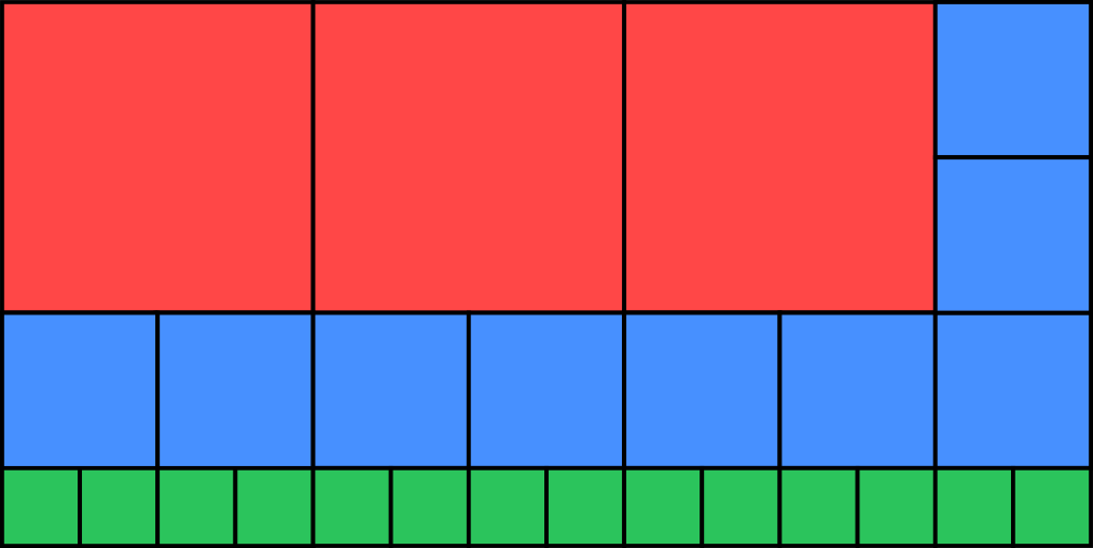
Capitalist indoctrinationGeometric intuition tells us that the optimal solution is obtained by being greedy:
We start from one corner and pack the cuboid with the biggest cube possible, then with the next smaller cubes, and so on. Basically, we keep adding layers of smaller and smaller cubes, like layers of an onion. The picture on the right illustrates this on a 2-dimensional cuboid of dimensions 14×7 with three ‘onion layers’ (note that each layer is at most 1 cube thick).
A lot of students implemented this and it works fairly well. The MC Sr’s very first solution of this was also an instance of this approach, but with a somewhat different spin: he computed the biggest cube that fits into the cuboid and cut out as many instances of it as possible starting from a corner. That leaves some leftover bits, which he then broke up into several cuboids, which he then decomposed recursively. That works, too, but it is very inefficient. None of the students (at least none in the Top 30) did this.
Instead, they simply carried around both the original cuboid and the sub-cuboid that they have already filled up, and added one ‘onion layer’ in each step.
While it seems intuitively obvious that this works, it really isn’t:
Why does the optimal solution need to have the biggest possible number of the biggest possible kind of cubes?
Why is it sufficient to put all the biggest cubes together in one corner?
The reader may think this is obvious, but geometric intuition is not a proof!
The crucial step seems to be to show that in any cuboid decomposition, the cubes can be moved around such that their corners are aligned (i.e. if the cube has side length d, all its coordinates are multiples of d). The MC Sr tried to come up with a direct proof for this but ultimately failed.
However, in his search of a proof, he actually found an (arguably simpler) approach for which the correctness argument is much easier, and which actually also makes it much easier to see why the above approach works. Several students also found this alternative approach, and we shall look at it now.
Peel and Shrink
Instead of starting with the biggest possible cubes, we can also start with the smallest possible cubes, namely those of side length 1. Geometric intuition tells us that we may as well assume that all these cubes of size 1 are in a single layer (i.e. at least one of their coordinates is the largest possible). For each odd dimension of the cuboid, we have a layer of width 1 of cubes of size 1 on one end, as illustrated by the following example of two 3-dimensional cuboids with dimensions 9×7×5 and 8×7×5:


The red cubes are the outermost layer; the blue part is the cuboid that remains after peeling off the outermost layer (note that the blue cuboid now has even dimensions).
We can then reduce the problem of computing the optimal decomposition to
computing the number of cubes of size 1 in the red part
computing an optimal decomposition of the remaining blue cuboid
The former can be done simply by comparing the volume of the original cuboid and the blue cuboid. The latter can be done by dividing all the dimensions by 2 (since all the dimensions are now even) and recursing. We can stop once our cuboid has length 0 in any dimension.
The elegance of this approach is demonstrated most strikingly by the following submission due to Frau Knapp:
decompose ds
  | 0 `elem` ds = []
  | otherwise = product ds - product [d - mod d 2 | d <- ds] : decompose [div d 2 | d <- ds]
This solution made it into the final round, but was not quite as fast as some of the more optimised solutions.
Still, this kind of solution is why the MC Sr loves Haskell! Short, concise, readable. This is the kind of solution you just want to print out, frame, and put on your office wall. The MC Sr hereby awards it with a Chef Kiss emoji  .
.
One of the winning solutions (namely the one by Herr Mio) uses the same basic approach, but with the crucial optimisation of caching the volume of the cuboid in a parameter to avoid having to compute two volumes in every recursive call.
decompose ds = decomposeRec ds (product ds) (length ds)

decomposeRec :: [Integer] -> Integer -> Int -> [Integer]
decomposeRec _ 0 _              =  []
decomposeRec ds size dim        = (size - shiftL newsize dim) : decomposeRec inner newsize dim
    where       newsize  = product inner
                inner    = map ( `shiftR` 1) ds
Since the arithmetic operations dominate the running time of the algorithm, this makes a big difference: his solution is about twice as fast as Frau Knapp’s. He also uses bit shifting instead of multiplying/dividing by 2, but that probably doesn’t make much of a difference – it’s quite possible that GHC does this anyway.
The MC Sr’s optimised solution is quite similar to that of Herr Mio:
decompose ds = let d = minimum ds in go (product ds) (d : delete d ds)
  where n = length ds
        go vol ds
          | head ds == 0 = []
          | otherwise    =
              let ds'    = map (`div` 2) ds
                  vol'   = product ds'
                  nCubes = vol - vol' `B.shiftL` n
              in  nCubes : go vol' ds'
The only real difference is another cheeky little optimisation that makes a very tiny difference: as a preprocessing step, the smallest dimension is pulled to the front of the list so that we do not have to check whether any dimension has become 0 after every step, but we can simply check whether the first one has become 0.
So why does this approach work? The MC Sr has a detailed proof for this, but to keep things short, he will only give you the key lemmas and sketch the proofs:
Every cuboid decomposition has an equivalent decomposition where all cubes of size ≥ 2 have even coordinates.
Proof: Consider a cube c of size ≥ 2 with odd coordinate x along some dimension (let’s say the left–right dimension to make things easier). Let the cube be chosen as far left as possible. Then all cubes adjacent to c on the left have an odd right coordinate and must thus be of size 1. Then we can simply move \(c\) to the left by 1 and all these cubes of size 1 to the right of \(c\). Repeat this process until there are no more cubes of size ≥ 2 with odd coordinates.Every cuboid decomposition has an equivalent or smaller decomposition where any cube of size 1 at coordinate \(x\) has \(x_i = d_i - 1\) with \(d_i\) odd for at least one \(i\). (i.e. all the cubes of size 1 are in a layer of width 1 at the far side, and only if the dimension is odd).
Proof: W.l.o.g. assume all cubes of size ≥ 2 have even coordinates. Suppose we had a cube \(c\) of size 1 at \(x\) with \(x_i < d_i - 1\) for all \(i\). Define \(\varepsilon_i = 1\) if \(x_i\) is even and \(\varepsilon_i = -1\) if \(x_i\) is odd. Then for each vector \(\delta \in \{0,1\}^n\) there exists a cube of size 1 at \(x + \delta \cdot \varepsilon\). We can replace these \(2^n\) cubes with a single cube of size 2. Repeat that process until no longer possible.An optimal decomposition of \((2d_1, \ldots, 2d_n)\) is obtained by taking an optimal decomposition of \((d_1, \ldots, d_n)\) and doubling the size of each cube (and vice versa).
Let \(\varepsilon\in\{0,1\}^n\). An optimal decomposition of \((2d_1+\varepsilon_1, \ldots, 2d_n+\varepsilon_n)\) is obtained by taking an optimal decomposition of \((d_1, \ldots, d_n)\), doubling the size of each cube, and adding a layer of cubes of size 1 in each dimension \(i\) for which \(\varepsilon_i = 1\) is odd. The other direction also works.
Global Optimisation 📉
Three students responded to the MC Sr’s challenge to prove the correctness of their approach. The first one submitted something in the same night that the exercise sheet was published, thinking that there would be dozens of submissions and that it would be vital that he be among the first. Alas, that anticipated deluge of proof submissions did not materialise! In the end, only one student submitted a convincing proof, and that was Herr Zehetbauer (PDF). He essentially proved the correctness of the greedy approach by looking at the problem globally (i.e. without any kind of induction) and with almost none of the tricky geometric reasoning in the MC Sr’s proof. His proof can be condensed down to this:
Proof. Consider a cuboid of dimensions \((d_1, \ldots, d_n)\). The maximum number of cubes of size \(2^i\) that we can have in a decomposition is \(b_i := \prod_j\, \lfloor d_j / 2^i\rfloor.\) That is the number we obtain by just greedily packing as many instances of that cube as possible next to each other, starting in one corner.
Now consider one particular decomposition that has exactly \(t_i\) cubes of size \(2^i\). One can easily see that \[b_i \geq t_i + 2^n t_{i+1} + 2^{2n} t_{i+2} + 2^{3n} t_{i+3} + \ldots\] since every cube of size \(2^{i+j}\) can be subdivided into \(2^{jn}\) cubes of size \(2^i\). Rearranging, we find that \[t_i \leq b_i - 2^n t_{i+1} - 2^{2n} t_{i+2} - 2^{3n} t_{i+3} + \ldots\] which gives us an upper bound for \(t_i\) depending on \(t_{i+1}\), \(t_{i+2}\), \(\ldots\). Herr Zehetbauer now claims that the optimal solution is obtained when all these inequalitities are equalities, i.e. starting with the biggest possible value for \(i\), we always let \(t_i\) be as big as possible.
To show the optimality of this greedy solution, introduce variables \[\Delta_i := b_i - t_i - 2^n t_{i+1} - 2^{2n} t_{i+2} - \ldots\] that measure the slack in each of the above inequalities (i.e. the greedy solution has \(\Delta_i = 0\) for all \(i\)). With some arithmetic (which the MC Sr leaves to the reader), one finds that \[t_i = b_i - \Delta_i - 2^n (b_{i+1} - \Delta_{i+1})\ .\] Recall that we want to minimise the total number of cubes, i.e. the sum of all \(t_i\). Summing over the previous equation for all \(i\), we find that: \[\sum_{i\geq 0} t_i = b_0 + (1-2^n)\left(\sum_{i\geq 1} b_i\right) + (2^n-1)\left(\sum_{i\geq 1}\Delta_i\right)\]Clearly, as the \(b_i\) are all fixed, this expression takes its minimum value iff \(\Delta_1 = \Delta_2 = \ldots = 0\). Furthermore, one can see that \(\Delta_0\) must be \(0\) as well because otherwise the decomposition would not even have the same volume as the cuboid. q.e.d.
While the MC Sr’s proof is perhaps a bit more anschaulich, he does like Herr Zehetbauer’s proof a lot because it is quite a bit simpler and avoids messy geometric reasoning. That’s a well-deserved extra large 🎓 emoji for Herr Zehetbauer, plus 10 bonus Wettbewerb points. Don’t spend them all at once!
Herr Zehetbauer’s proof directly yields a very simple algorithm for computing the optimal solution: we need only set all the \(\Delta_i = 0\) in the above equations and obtain \(t_i = b_i - 2^n b_{i+1}\), and the \(b_i\) are easily computed. A few students also implemented this approach; the most concise one being the winning solution by Frau Biltzinger:
decompose ds =
  let mult = 2 ^ length ds
      lowest = minimum ds
  in  if null ds || lowest < 1 then [] else
      snd $ mapAccumR (\prev this -> let prod = product this in (prod, prod - mult * prev)) 0 $
      take (log2 lowest + 1) $ iterate (map (`div` 2)) ds
Conclusion
There were a number of very different approaches again this week, quite a few of which were on par with the MC Sr’s (which makes him happy), but none of which could really outperform his (which also makes him happy, especially after the diaster with his Sudoku solver in week 3 – yes, the MC Sr is vain 😉).
It seems that all the approaches that the MC Sr saw in the Top 30 compute the greedy solution one way or another. For higher dimensions, the running time is dominated completely by the arithmetic operations since the numbers involved become absurdly large. This completely eclipses most other differences in the implementations such as the choice of data structures or typical performance killers like appending to the end of a list instead of the beginning. This is why the Top 30, especially, the first third, are very close together.
Interestingly, for quite some time after the MC Sr had originally decided to pose this as a homework problem, he did not know how to prove his approach correct, and his best algorithm was not any of the fast and simple solutions, but the much more complicated one where one greedily cuts out as many big cubes as possible and then breaks the remaining bits of the cuboid into up to n new cuboids on which one then recurses. This has an abysmal exponential running time!
He did eventually find the fast and simple ‘peel-and-shrink’ solution, and the correctness proof soon followed. The MC Sr spent quite a bit of time improving his very inefficient first algorithm and trying to prove it correct. When he then found the much simpler ‘peel-and-shrink’ solution and the corresponding proof, it felt like an epiphany and he was satisfied that he now understood the problem completely. But in the end, while looking at the student submissions (first and foremost Herr Zehetbauer’s proof), it turns out that there was more to learn yet! He was initially quite worried that the exercise might be too difficult for the FPV students, but clearly that was not a problem.
Interestingly, the MC Sr also found indications that two students used self-written QuickCheck tests on some of their functions. That is commendable! Additionally, at least one student also employed profiling on their code to find out which parts are the most expensive. That can be very useful, although in this particular case, a different, simpler algorithm would have gone much further than such incremental improvements. But that is easy for the MC Sr to say now – hindsight is 20/20, after all. (For what it is worth, the MC Sr had also wasted a lot of time dotting the i’s and crossing the t’s in his first solution before scrapping it completely in favour of the faster and simpler one.)
What did we learn this week?-
Students do surprise the MC Sr again and again (positively)!
-
Like a Sudoku solver, humans sometimes get stuck chasing down a wrong path. As difficult as it may be, sometimes one simply has to reset one’s brain, start from scratch, and try some radically different ideas to find the best solution. The MC Sr knows this, but should perhaps try to keep this in mind more.
-
Often, looking for a simple and rigorous proof can actually lead you to a simpler, more elegant, and faster algorithm.
-
Many FPV students seem to have no problems thinking in 10000 dimensions.
-
Their enthusiasm for proofs seems to have waned somewhat though. What a pity! This means even more respect for Herr Zehetbauer is in order.
-
GHC does not like emojis. At least not always. Herr Ouyang submitted a solution full of functions like this:
(😯) :: [Integer] -> [Integer]
(😯) (0 : _) = []
(😯) (❓)@((🦉) : _) = (❗) 🤔 reverse
  where
    (📖) = (❓) 🤔 length
    (👏) = (🦉) 🤔 log2
    (❗) = ((❓) 😘 (🌲) (📖)) (👏)
For some reason, this does not compile in the MC Sr’s test environment (
lexical error at character '\129300'). Not sure what is going on here – perhapsstackuses a different GHC version? The MC Sr was too lazy to investigate. Luckily, Herr Ouyang had the good sense to include an alternative version without funky unicode symbols that worked just fine. Apparently he did not want trolling to get in the way of a good Wettbewerb result after all! -
What is it with the MC Jr Kappelmann and his strange obsession with CSS snowflakes…
Ranking
The table lists the highest benchmarking stage that the student reached and the time that their solution required in that stage. Of course, only times of students in the same stage can really be compared.
| Rank | Name | Stage | Time | Points |
|---|---|---|---|---|
| 🥇 | Maren Biltzinger | 6 | 46.96 s | 30 |
| 🥇 | Kilian Mio | 6 | 47.16 s | 30 |
| 🥉 | Julia Bauernfeind | 6 | 45.71 s | 28 |
| 4. | Simon Longhao Ouyang | 6 | 44.95 s | 27 |
| Salim Hertelli | 6 | 46.65 s | 27 | |
| Martin Felber | 6 | 46.00 s | 27 | |
| 7. | Felix Zehetbauer 🎓 | 6 | 51.45 s | 15 + 24 |
| Alexander Steinhauer | 6 | 51.74 s | 24 | |
| 9. | Manuel Kühnle | 6 | 48.91 s | 22 |
| 10. | Kevin Pfisterer | 6 | 70.53 s | 21 |
| 11. | Sophia Knapp |
6 | 90.11 s | 20 |
| 12. | Patryk Morawski | 6 | 89.97 s | 19 |
| Nils Cremer | 6 | 92.26 s | 19 | |
| 14. | Simone Theresia Zügner | 6 | 86.86 s | 17 |
| Nils Imdahl | 6 | 89.88 s | 17 | |
| 16. | Constantin Wild | 5 | 16.94 s | 15 |
| 17. | Arcangelo Capozzolo | 5 | 34.94 s | 14 |
| 18. | Luis Bahners | 5 | 73.37 s | 13 |
| 19. | Matthias Jugan | 5 | 70.95 s | 12 |
| 20. | JiWoo Hwang | 5 | 74.24 s | 11 |
| 21. | Simon Kammermeier | 5 | 105.39 s | 10 |
| 22. | Eddie Groh | 5 | 119.39 s | 9 |
| 23. | Benjamin Defant | 5 | 295.07 s | 8 |
| 24. | Armin Ettenhofer | 4 | 495.39 s | 7 |
| 25. | Tianze Huang | 3 | 28.92 s | 6 |
| 26. | Jakob Florian Goes | 3 | 43.13 s | 5 |
| 27. | Florian Hübler | 3 | 39.18 s | 4 |
| 28. | Vitus Hofmeier | 3 | 67.56 s | 3 |
| 29. | Olha Dolhova | 3 | 81.76 s | 2 |
| 30. | Simon Pannek | 3 | 100.93 s | 1 |
Week 6
🎵🎵 Hello, this is the MC Jr Jr speaking singing 🎵🎵
The MC Jr Jr originally meant to use his time machine to get the blog entry released earlier but apparently the time machine broke and it instead transported him forward in time. Or maybe it was just the Christmas holidays that transported him forward in time without getting anything done, who knows?
As fortune wants it, the only musical Wettbewerb will be evaluated by the MC with the least musical expertise (two are guitar players and one is an excellent accordion player, or so he’s told).
Then again, he is quite the fan of electronic music and dabbled a bit in DJ-ing himself.
The MC Jr Jr was very pleased that some students took it further than just twiddling with some effect knobs and putting on a good show by designing custom instruments or even composing their own songs.
But even minor changes granted you a spot on the board this week as only 19 students of over 300 with WETT tags did change the template.
Here, a shoutout to the amazing FPV tutors is in order since they helped the MC Jr Jr to sift through all those submissions.
Enough talk, let’s see hear what our aspiring students of the Haskell school of music came up with.
Instruments
Great instruments are essential to realise the potential of a composition. Many students recognised this and came up with their own instruments to replace those given in the template. A notable example for this is the Song of Storms which benefits from a more organic organ to bring it closer to the original. Compare the version produced by the model solution with that of Herr Philipp Wittmann or Herr Benjamin Defant. In fact, both only added this instrument and they used the same approach of approximating the sawtooth wave using some summands of its fourier series.
Instead of synthesising instruments, two students used pre-recorded samples of instruments.
Whereas Herr Max Lang lazily read the sample from a file using unsafePerformIO (🔴🔵🔴🔵🔴🔵), Herr Julian Sikora was more creative and analysed his samples, some of which he even recorded himself, using the fourier transform.
The fourier transform divides a given signal into its component frequencies and their amplitudes.
He then extracted the most significant frequencies by amplitude and synthesised them with our Haskell framework, essentially reversing the fourier transform.
Herr Sikora remarks that this only approximates the original signal and therefore the technique works best with instruments that don’t produce a large amount of different frequencies.
For example, a violin works well because it only has 4 strings but it is difficult to reproduce the sound of a human voice.
Although the MC Jr Jr feels the urge to chastise Herr Sikora’s use of Python (gasp) for the fourier transform, he will give him a pass on account of his elegant approach.
Effects
To make the soundscape more lively, we can play around with effects, some of which will be presented below.
Bitcrusher According to Wikipedia this effects combines two methods to reduce audio fidelity: sample rate reduction and resolution reduction. The first part of the effect is easy enough to implement as Herr Gumbart demonstrates:
bitCrunch [] = []
bitCrunch (x:_:xs) = x:x:bitCrunch xs
bitCrunch (x:xs) = x:bitCrunch xs
Simple and elegant! There were also some variations like skipping every second sample (instead of duplicating it like above). The second part was implemented very succinctly by Frau Biltzinger:
reduceResolution n = map (\x -> fromInteger (truncate (x * n)) / n)Since our samples are assumed to be between \(-1\) and \(1\), we can multiply by \(n\), throw away everything after the comma, and divide by \(n\) again to obtain a signal whose amplitude only has \(2n\) different values. Unfortunately, nobody seems to have combined the two components into one effect.
Echo and reverb Since real instruments are not played in a vacuum, one usually adds effects that simulate the conditions of a physical location, which also makes them sound more natural. To simulate a large room, one can add an echo: we pad the signal with silence in front and then mix it with the original signal. As an example, listen to the echo that Herr Bahners implemented:
echo :: Seconds -> DSPEffect
echo t xs = hilf xs (replicate (samplesPerSecond t) 0.0) []
  where
    ss = (replicate (samplesPerSecond t) 0.0) ++ xs
    hilf :: SampledSignal -> SampledSignal -> SampledSignal -> SampledSignal
    hilf [] _ _ = []
    hilf (x:xs) (y:ys) sx = let nxt = (0.7*x + 0.3*y) in nxt : hilf xs ys (nxt:sx)
    hilf xs [] sx = hilf xs (reverse sx) []
A simple reverb can be implemented as several echoes occuring within a short timespan after the original sound. More abstracly, Herr Schmitz implemented reverb in terms of a convolution where each output sample is the result of a linear combination of the preceeding samples. The key difference between difference between echo and reverb is, according to Wikipedia, that echo is heard between \(50\) and \(100ms\) while the sound reflections of reverb arrive in under \(50ms\). This is also reflected in Herr Schmitz’ code as he combines the current sample and 3 preceeding samples with a distance of \(500s / 48000 \approx 10ms\):
convolve :: (Num a) => [a] -> [a] -> [a]
convolve hs xs = map (sum . zipWith (*) (reverse hs)) (init $ tails ts)
  where
    pad = replicate ((length hs) - 1) 0
    ts  = pad ++ xs

reverb = convolve ([1.0] ++ replicate 500 0.0 ++ [0.8] ++ replicate 500 0.0 ++
                   [0.6] ++ replicate 500 0.0 ++ [0.1])
Listen to the result. Herr Lang went even further and tried his hands on implementing a Schroeder reverberator to produce this tune.
Tremolo and chorus
Another interesting effect that emulates aspects of real instruments is the tremolo effect.
It is often employed when playing string instruments, e.g. the violin, and is characterised by a rapid variation of amplitude or frequency.
A variant that modulates the frequency was kindly provided by Frau Knapp.
Again, Frau Knapp impresses with well structured, readable, and concise code .
{- TREMOLO
  time: the time of one repetition of the modulation in seconds
  amount: 1 -> big change in pitch, 0 -> small change in pitch

  Note: This Tremolo effect is implemented by first dividing the given track in chunks of
    the length of each repetition of the effect, then each of these chunks is split in 2 parts again,
    the first part will be shortened by deleting every nth sample (increasing the frequency).
    the second part is lengthened by duplicating every nth sample (decreasing the frequency)
-}
tremolo :: Seconds -> Double -> DSPEffect
tremolo time amount track = concatMap (addTremolo sampleCount) (splitEvery (samplesPerSecond time) track)
  where
    sampleCount = round ((1 - amount) * 10) ^ 4

addTremolo :: Int -> SampledSignal -> SampledSignal
addTremolo amount track = deleteEvery amount (fst parts) ++ duplicateEvery amount (snd parts)
  where
    parts = splitAt (div (length track) 2 + amount) track

splitEvery :: Int -> [a] -> [[a]]
splitEvery _ [] = []
splitEvery n list = next : splitEvery n rest
  where
    (next, rest) = splitAt n list

duplicateEvery :: Int -> SampledSignal -> SampledSignal
duplicateEvery _ [] = []
duplicateEvery n xs = head xs : take n xs ++ duplicateEvery n next
  where
    next = drop n xs

deleteEvery :: Int -> SampledSignal -> SampledSignal
deleteEvery _ [] = []
deleteEvery n xs = take (n -1) xs ++ deleteEvery n (drop n xs)
She then uses tremolo to implement a chorus effect which creates the illusion of multiple instances of one instruments playing in concert. Listen here to appreciate the effect! The code speaks for itself:
{- CHORUS
  tempo: how much the added track is delayed (see note)
  amount: 1 -> only wet signal, 0 -> only dry signal

  Note: This chorus is implemented by mixing the original signal with a track that
  has been slightly delayed and has a slight tremolo effect applied to it.
-}
chorus :: Seconds -> Double -> DSPEffect
chorus tempo amount track = mixTracks [track, wetSignal] [1 - amount, amount]
  where
    silence = replicate (samplesPerSecond tempo) 0.0
    wetSignal = tremolo 0.3 0.5 (silence ++ track)

mixTracks :: [SampledSignal] -> [Double] -> SampledSignal
mixTracks trks vols = mix $ zipWith (\trk vol -> map (* vol) trk) trks vols
Miscellaneous After painstakingly customising the instruments and coding up a few effects to spice things up, you may want to bask in the glory of your composition only to find out that the audio file you produced has unpleasant popping. You can hear this here or here. A probable cause for this is that the ADSR-envelope from the template is not very flexible: the length of attack, decay, sustain, and release is absolute. If the length of notes varies, it might lead to short notes being over before the release phase is over. The amplitude suddenly drops to zero at the end of the note which results in popping. Herr Lang deals with this by scaling the ADSR parameters to the length of the signal if the length of the envelope exceeds the length of the signal.
Songs
As per the exercise sheet, the students were allowed to provide their own MIDI files and some happily took that opportunity. Owing to the season, some Christmas songs were in order: “Carol of the Bells”, “Frosty the Snowman”, and a song that may be accurately called “We Wish You a Farty Christmas”. Additionally, we seem to have a trotse Nederlander among our Wettbewerbers indicated by Herr Harmsen’s use of the national hymn of the Netherlands. There is also a little something for fans of algoraves in the form of remixes of deadmau5 and Avicii songs. The obligatory Rickroll is kindly provided by Herr Bahners, which would otherwise have been sorely missed by the MC Jr Jr. To great delight of the MC Jr Jr, there were also original compositions by Frau Knapp, Herr Schmitz, and Herr Gockel. For going above and beyond to satisfy the demanding MCs, the MC Jr Jr rewards them with the prestigious 🎼-emoji and 5 bonus Wettbewerb points. The table below contains thoses submissions that provided their own MIDI file including a reference to the original/another interpretation of the song.
| Name | Song | Interpretation | Reference |
|---|---|---|---|
| Sophia Knapp | Haskell Song | - | |
| Malte Schmitz | Great Hall | - | |
| Markus Gockel | Entspannung | - | |
| Jonas Alexander Lauer | We Wish You a Merry Christmas | Link | |
| Markus Gumbart | Carol of the Bells | Link | |
| Nina Tarina Jasmin Cordes | Frosty The Snowman | Link | |
| Nils Harmsen | Wilhelmus (National Anthem of the Netherlands) | Link | |
| Julian Sikora | Nadia Ali - Rapture (Avicii Remix) | Link | |
| Maren Biltzinger | deadmau5 - 2448 | Link | |
| Luis Bahners | Rick Astley - Never Gonna Give You Up | Link |
Evaluation
Finally, we come to the results of this week’s Wettbewerb.
Since music is an art, the beauty is of course in the eye ear of the beholder and any scoring mechanism is necessarily highly subjective.
To even things out a bit, the scores are not given by the MC Jr Jr alone but are instead decided by a Rat of the MCs consisting of the MC Sr, MC Jr, and the MC Jr Jr, each one giving a score from 1 to 10.
In addition to that, the MC Jr Jr also scored the code, again on a scale of 1 to 10, in terms of technical effort and elegance.
The final score consists of the sum of the MCs scores and two times the code score.
For reference, here are the provided songs as interpreted by the model solution: mario.mp3, star.mp3, song_of_storms.mp3.
As a little Schmankerl on top, we will provide the top 3 with some teaching material, namely the book “The Haskell School of Music”. Stay tuned and check your eMailbox.
Conclusion
What did we learn this week?
- Generating sounds in Haskell and adding simple effects is surprisingly simple.
- Adding duplication and interference in the form of reverb, tremolo, and chorus goes a long way to produce a rich soundscape.
- Going from generating sounds to generating music is still hard as evidenced by the low number of submissions this week.
| Rank | Name | Audio | Lukas | Manuel | Kevin | Tech | Sum | Points |
|---|---|---|---|---|---|---|---|---|
| 🥇 | Sophia Knapp 🎼 | 10 | 10 | 10 | 10 | 50 | 30 + 5 | |
| 🥈 | Max Lang | 9 | 9 | 9 | 10 | 47 | 29 | |
| 🥉 | Malte Schmitz 🎼 | 8 | 7 | 7 | 8 | 38 | 28 + 5 | |
| 4. | Julian Sikora | 8 | 6 | 8 | 7 | 36 | 27 | |
| 5. | Luis Bahners | 9 | 7 | 7 | 6 | 35 | 26 | |
| 6. | Markus Gumbart | 8 | 6 | 7 | 6 | 33 | 25 | |
| Nina Tarina Jasmin Cordes | 7 | 8 | 8 | 5 | 33 | 25 | ||
| 8. | Maren Biltzinger | 6 | 5 | 5 | 5 | 26 | 23 | |
| 9. | Florian Hübler | 5 | 4 | 4 | 6 | 25 | 22 | |
| Markus Gockel 🎼 | 6 | 4 | 5 | 5 | 25 | 22 + 5 | ||
| 11. | Simon Longhao Ouyang | 5 | 4 | 5 | 5 | 24 | 20 | |
| 12. | Xuemei Zhang | 5 | 4 | 5 | 4 | 22 | 19 | |
| 13. | Severin Schmidmeier | 4 | 3 | 4 | 5 | 21 | 18 | |
| 14. | Josef Schönberger | 3 | 2 | 3 | 6 | 20 | 17 | |
| 15. | Nils Harmsen | 6 | 4 | 5 | 2 | 19 | 16 | |
| Julian Pritzi | 3 | 5 | 5 | 3 | 19 | 16 | ||
| 17. | Benjamin Defant | 5 | 5 | 4 | 2 | 18 | 14 | |
| 18. | Philipp Wittmann | 4 | 3 | 6 | 2 | 17 | 13 | |
| 19. | Jonas Alexander Lauer | 4 | 1 | 3 | 4 | 16 | 12 |
Week 7
Hullo everyone, this is the MC Sr again. Or perhaps rather, as of 21 January, Dr. rer. nat. MC Sr? Well, not quite – there is still some bureaucracy that has to be done before he can actually call himself that, but he did pass his PhD exam! 🥳
But enough partying. There is work to be done! The MC Jrs are busy coming up with the most torturousfair and reasonable exam questions possible, so they delegated the enormous burdenpleasure of evaluating the solutions for the Virus Game task to the tutors and that of writing the blog article to the MC Sr. Unfortunately, the MC Sr knows virtually nothing about the game in question, nor does he know anything about how to write AIs for games in the first place. So with that in mind, take his writings here with a grain of salt. Luckily, the tutors seem to know more than he does and provided a table that lists the approach that each submission took, plus some further brief comments. It is this evaluation that the MC Sr will base this blog entry on.
For those of you who did not figure it out already, the virus game is simply a relabelled version of the Android game called Chain Reaction. A brief explanation of the rules and one possible heuristic can be found on Brilliant.
The important thing when writing an AI for a combinatorial game with alternating moves is to find a good way to rank possible moves, i.e. to figure out what the best possible move is (Captain Obvious strikes again). In finitely-branching two-player games of finite length (such as chess, Go, or indeed Chain Reaction) one of the two players can always force a win (or a draw, if the game has draws, which Chain Reaction does not).
This can be shown by induction over the (finite) game tree, whose nodes are the valid game states, with the root node being the empty board and the leaves being non-empty boards in which all the orbs belong to one player: in any game state S where it is player A’s turn, there are finitely many successor states. By induction hypothesis, in each of these, one of the two players can force a win. If player B can force a win in all of the successor states, then player A cannot win in state S. If, on the other hand, there is a successor state S’ in which player A can force a win, then player A can also force a win from S by playing a move that leads to the new state S’.
This proof is constructive in the sense that one can derive an actual algorithm from it that computes (in finite time) which player can force a win and how: run a DFS on the game tree and determine, bottom up, who can force a win from each state. In practice, however, this is completely impractical: even if there are only a few moves possible in every game state, the number of possible states grows exponentially with the length of the game, so that this only works for relatively simple games such as Tic-tac-toe (or ‘noughts and crosses’ for those who, like the MC Sr, prefer British English).
For games with large game trees (such as ours), this is clearly not feasible, so one has to look at more practical approaches to figure out what the best move in a given situation is. The easiest way is to just look at the immediate consequences of the move: one figures out some kind of scoring heuristic for judging how ‘good’ a game state is – e.g. the difference between the number of orbs owned by you and that of the other player. The students used various heuristics; all of them (as far as the MC Sr can see) basically amount to counting the player’s orbs as +1 and the opponent’s orbs as -1, with some additional weighting, such as counting orbs at the edge of the board double or giving a penalty to orbs that can be taken over by the opponent in the next move. Several people also implemented the heuristic from Brilliant.
A more refined approach explores not just the immediate consequences of the move, but some of the next few layers of the game tree as well: one can e.g. go through all the possible follow-up moves by the opponent and then apply the heuristic to these to figure out what the worst possible game state (according to the heuristic) is that the opponent can achieve. The move for which this worst game state is best is then the move that we make. One can go further than just one layer, of course, but the pattern is always the same: in each layer where it is player B’s turn, we take the move that leads to the worst state; in each layer where it is player A’s turn we take the one that leads to the best state. This is called the Minimax approach. An optimisation of this is called α–β–pruning. It leads to the same result but discards certain irrelevant parts of the game tree quickly so that one can explore the tree more deeply in the same amount of time.
Such game AIs are similar to some of the other tasks (solving Sudokus, resolution proving, SAT solving) that we have seen this year or in earlier years in that some performance optimisations rarely lead to great improvements while high-level conceptual optimisations can lead to results that are orders of magnitudes better. Implementing fancy α–β–pruning and optimising it to run four times faster than that of your opponents is practically useless if they have a better underlying heuristic than you do. This is shown in the table: almost all the top-ranked students all employ α–β–pruning, but there are quite a few α–β–pruning people in the lower ranks as well.
That said, Herr Markus, who won the competition this week, did so by optimising the living daylights out of his α–β–pruning in over 2000 lines of code. The most important optimisations are probably caching of interesting moves in the global state and various heuristics (all explained in the massive MCCOMMENT at the beginning of his submission). However, he also employed a number of other, more low-level optimisations:
using the
STmonad for destructive imperative updatesinlining annotations and rewrite rules
representing game states as three 64-bit integers using some bit magic
The MC Sr does not know how big the performance gain from these actually is (the inlining/rewrite rules probably have little effect, if any). Herr Markus also enabled 14 different compiler extensions (including some the MC Sr had never heard of). In any case, something must have helped since Herr Markus won, despite his game valuation heuristic apparently being relatively simplistic: difference of the number of orbs of both players, with a bonus for critical orbs (at least if the MC Sr interpreted the code correctly – it is somewhat difficult to tell). Remarkably, Herr Markus’s strategy is also the third-fastest among the Top 19 (and almost tied with the second-fastest). There are many strategies that take one order of magnitude more time but still do not perform as well.
Herr Schmidmeier (in second place) uses the standard heuristic with additional penalties for endangered orbs and bonuses for critical cells and corners. He also uses a hard-coded order in which possible moves are considered in the hope of finding a good move leading to a cutoff in the α–β–pruning earlier (a common approach).
Herr Lang (in fourth place) caches the scores for moves in the game tree to avoid recomputing them. The MC Sr is not sure whether that is actually necessary (i.e. if recomputing scores is something that happens in the first place), but he did not think about it very much. In any case, due to lazy evaluation, doing this will probably not hurt much either. It might lead to increased memory usage and thus also to worse performance due to increased garbage collection – but since Herr Lang did very well in the ranking, it probably does not. Still, the MC Sr is curious whether the performance actually would be worse without the caching.
The MC Sr would love to say more about the other solutions, but time is running out (this blog entry must be ready for the lecture closing ceremony, after all) and the tutor’s evaluation does not turn up any hugely interesting differences between the student submissions. It seems that they are all implementations of either standard α–β–pruning or plain Minimax, with varying heuristics. So with that, let us finish up and get to the ranking.
So what have we learnt this week?
Still a student at heart, the MC Sr likes to procrastinate unpleasant tasks until the very last moment. Not that writing these blog entries is unpleasant in general – but it is very work-intensive, and it is very difficult in instances like these were he is not familiar with the subject matter and did not even attempt to solve the task himself. He hopes he still did an all right job at writing this!
While the MC Sr had trouble finding adequate games for the Wettbewerb even back in 2014 (especially ones where you don’t copypastable strategies all over the web), the MC Jrs seem to find interesting ones year after year without any trouble.
This semester’s FPV lecture was of remarkably high quality. The MC Jrs and the tutors went above and beyond with the quality of some of the exercises (such as this one) and especially all the other things they organised (such as the programming competition and the workshops). The MC Sr is very proud of them. (And a bit appalled at how these young whippersnappers managed to upstage him!)
Many of the student submissions of this year were also of remarkably high quality. Κῦδος to our Wettbewerblinge as well! Do keep the Chair of LoVe in mind during the remaining years of your studies! The Semantics and Functional Data Structures courses are good follow-up Lehrveranstaltungen to FPV – and highly addictive (that’s how Prof. Nipkow got his army of MCs, after all).
The meme game on Zulip was also, again, excellent. The MC Sr’s proudest achievement this semester is clearly that one student called the FPV-Übungsleitung ‘Meme Gods of TUM’ in the lecture evaluation. He is contemplating putting this on his CV.
Note: The results in this table differ slightly from the website since all the matches of the Top 48 were resimulated again (10 times each) for the final evaluation. You can find all results here.
| Rank | Name | Wins | Approach | Points |
|---|---|---|---|---|
| 🥇 | Tobias Markus | 879 | AB+ | 30 |
| 🥈 | Severin Schmidmeier | 831 | AB | 29 |
| 🥉 | Florian Hübler | 804 | AB | 28 |
| 4. | Max Lang | 803 | AB | 27 |
| 5. | Dominik Weinzierl | 795 | Minimax | 26 |
| 6. | Manuel Pietsch | 792 | AB | 25 |
| 7. | Felix Zehetbauer | 782 | AB | 24 |
| 8. | Philip Haitzer | 756 | Minimax | 23 |
| 9. | Maren Biltzinger | 746 | Minimax | 22 |
| 10. | Paul Volk | 741 | Minimax | 21 |
| 11. | Benjamin Defant | 717 | Minimax + Heuristic? | 20 |
| 12. | Alexander Steinhauer | 716 | Minimax | 19 |
| 13. | Patryk Morawski | 694 | AB | 18 |
| 14. | Manuel Kühnle | 662 | AB | 17 |
| 15. | Sophia Knapp | 655 | Heuristic | 16 |
| 16. | Joong-Won Seo | 621 | AB | 15 |
| 17. | Martin Felber | 615 | Minimax | 14 |
| 18. | Skander Krid | 614 | AB | 13 |
| 19. | Jakob Florian Goes | 558 | Minimax | 12 |
| 20. | Daniel Schwermann | 556 | Heuristic? | 11 |
| 21. | Johannes Stöhr | 535 | 10 | |
| 22. | Jakub Stastny | 515 | Minimax | 9 |
| 23. | Maximilian Schalk | 499 | Minimax | 8 |
| 24. | Eddie Groh | 496 | Heuristic | 7 |
| 25. | Fabian Wenz | 437 | 6 | |
| 26. | Markus Englberger | 420 | Minimax | 5 |
| 27. | Flavio Principato | 412 | 4 | |
| 28. | Jalil Salamé Messina | 387 | Minimax | 3 |
| 29. | JiWoo Hwang | 360 | 2 | |
| 30. | Benjamin Holl | 352 | 1 |
Week 8
Hello my fellow formal logic connoisseurs 🍷 It has been a long time since the MC Jr last has been chosen to write a holy Wettbewerb blog entry. But the words of logic shall never pass his ears without reaction. And so he awakened to once again share his views on the science of truth.
As you know, the Wettbewerb’s evaluation order is unspecified, and so this time, you are getting the results for week 8 before those of week 6 and 7. But the threads that are proccessing week 6 and 7 are already running!
This week, the MC Jr kindly asked for the submission of efficient propositional resolution provers. Much time can be spent on optimising the task at hand as presumably many of you know by now. There’s an abundance of existing literature and ongoing research about this topic. To get you started, the MC Jr gave you some pointers for optimisations on the exercise sheet, but much more can be done. Let’s see what treasures this week’s Wettbewerb holds for us.
Test 0: Essentials
A striking number of Wettbewerb submissions – way beyond 30 – landed on the MC Jr’s laptop. However, many of those merely seemed to try to sponge some sweet Wettbewerb points in case of a lacking number of submissions. So as a first step, the MC Jr had to trenn die Spreu vom Weizen, that is to find the 30 submissions worthy of deeper investigation.
In all what follows, the MC Jr will work according to the principle of greatest transparency. So here are the rules:
- All test case parameters, including used QuickCheck (QC) seeds, will be listed in a table. The used stack resolver is lts-16.12.
- The used generators can be found in the following file: Generators.hs.
You can pass seeds to QuickCheck as follows:
QC.quickCheckWithResult QC.stdArgs{QC.replay = Just (mkQCGen yourSeed, 0)}. - The test machine is run by an Intel i9-9880H CPU @ 2.30GHz with 32GB of RAM.
- All submissions were compiled in extreme mode
-O2. 🔥 - Some evaluations were run in parallel if given input formulas were sufficiently small. More complicated test cases were run sequentially for the sake of having a fair testing environment.
- There will be 4 test suites, each stressing the provers in a different kind of way. Each test suite will be assigned a priority number, indicated by the number of ❗.
- There will be a ranking for each test suite. The ranking will be multiplied by the priority of the test suite, resulting in a test suite score.
- To obtain a test suite ranking, increasingly larger problems will be fed to the provers in separate runs. Students with very similar runtimes will share a spot in the ranking.
- The final score of this Wettbewerb is the sum of the test suite scores.
Sounds complicated? Don’t worry. It will become clear once we start. To run the evaluations, the MC Jr used the shiny, new Wettbewerbsauswertungsprogramm 🌠 written by the most senior of the MC’s, which, to his great surprise, worked way better than the file extension of the program (*.sh) suggests. Kudos to him.
So let’s get started with round #1. The MC Jr used the following parameters to create 100 tiny, random formulas.
| Generator | Timeout [seconds] | #Test Cases | QC Seed | Freq. Pos Vars | Freq. Neg Vars | Max. Var | Max. Clause Size | Max. #Clauses |
|---|---|---|---|---|---|---|---|---|
genEConjForm1 |
10 | 100 | 13 | 1 | 1 | 3 | 3 | 20 |
Innucous as they are, those generated formulas already ended the Wettbewerb for many students,
narrowing down the number of worthy candidates to 32.
But thanks to Peano, we know that 32 > 30, and so a second round is needed to narrow down the list of candidates just a bit further:
| Generator | Timeout [seconds] | #Test Cases | QC Seed | Freq. Pos Vars | Freq. Neg Vars | Max. Var | Max. Clause Size | Max. #Clauses |
|---|---|---|---|---|---|---|---|---|
genEConjForm1 |
10 | 100 | 13 | 1 | 1 | 3 | 8 | 8 |
Exactly 3 students failed this round: One of them, Herr Frölich, just took too much of a relaxed approach when faced with these slightly larger clauses. The other two dropped out due to the cardinal sin of providing wrong proofs:
FAIL by Thu Ha Dao
*** Failed! Falsified (after 8 tests):
[[~1,3,~2],[3,3,~3,2,1],[1,1,2],[~3,2],[1,1,~2,~2],[~2,2,2,~3,1,~3,~2,2],[2,~1,1]]
Model ["2","2"]
is not a valid proof for the given formula
FAIL by Felix Zehetbauer
*** Failed! Falsified (after 11 tests):
[[~2,~2],[2,1],[3,3,~2,~3],[~2,1,1],[~1,3,~1,2,~3,~1,~2],[~3,3,3,~1,1],[3,~1,~1],[1,~2]]
Model ["2","2","3","1"]
is not a valid proof for the given formulaLesson learnt: never trust a system unless
- It hands you a proof.
- You have a proof-checker.
- You have a proof that your proof-checker is correct.
- You have someone that verifies the proof that your proof-checker is correct.
- …
Or simply verify the system with Isabelle. But that’s a story for another lecture… Anyway, here are the 29 submissions that already made it into the finals:
Aaron Tacke, Benjamin Defant, Björn Brandt, Cara Dickmann, Christiane Kobalt, Christoph Starnecker, Dominik Weinzierl, Eddie Groh, Felix Brandis, Felix Krayer, Flavio Principato, Florian Hübler, Florian Schmidt, Jakob Florian Goes, Jakub Stastny, Jalil Salamé Messina, JiWoo Hwang, Jonas Benjamin Goos, Julian Pritzi, Luis Bahners, Markus Englberger, Max Schröder, Niclas Schwalbe, Niklas Lohmann, Robert Imschweiler, Simon Longhao Ouyang, Sophia Knapp, Tobias Markus, and Vitus Hofmeier.
Now, the MC Jr is a forgiving man (and he needs 30, not 29, students for the finals). So he decided to let one of the three failed – partly not so sound – submissions continue. He used the following parameters to settle the case.
| generator | timeout [seconds] | #test cases | qc seed | freq. pos vars | freq. neg vars | max. var | max. clause size | max. #clauses |
|---|---|---|---|---|---|---|---|---|
genEConjForm1 |
20 | 100 | 13 | 1 | 1 | 5 | 8 | 15 |
And while Herr Frölich’s submission again had to be stopped by the merciless timer, and Frau Dao’s solver returned another faulty proof, Herr Zehetbauer’s prover does not seem to be so inconsistent in general, returning 100 correct proofs in the blink of an eye. For all upcoming test suites, the MC Jr hence decided to disqualify submissions with faulty answers on a per test suite-basis.
As a note to Frau Dao: the MC Jr is very sorry that your prover failed to make it into the finals as it seems like quite some time was spent on your submission. As an advice: your code seems very non-modular and rather complicated. You should improve your code in that direction. Modularity and clarity are the best way to avoid bugs! 🐞
Now, what did it take to make it into this week’s finals? What were the essential optimisations? The bare minimum, it appears, were the following insights:
- If want to you use lists as sets, you better keep the invariant that they don’t store duplicates.
This can easily by achieved by calling
nub. Why does that matter? Well, the main issue of resolution provers is that they are saturation based and create huge working sets. The larger your sets, the more work you have to do. We hence want to keep these sets small. Treating, for example,[1],[1,1],[1,1,1],… as separate clauses surely won’t help in that regard. What is worse, it can even lead to non-termination!
Consider the unprocessed input formula[[-1,1,2],[-1,1,2,2]], where negative/positive numbers correspond to negative/positive literals. Resolving both clauses leads to a new clause[-1,1,2,2,2], and resolving that clause with any of the initial ones yet adds another2ad infinitum! Ouch! 🤕 - Another insight that many students had is that checking for set equality
s1 == s2using our list-based encoding is very slow but done very frequently – at least in many of the submitted provers. To speed this up, we can sort each list once when inserting it into our clause sets. Checking for set-equality then reduces to checking list-equality.
Besides, keeping things sorted will also help with selecting short clauses, as we will discuss further below. - Finally, we can remove tautological clauses to reduce the size of our clause sets even further.
A propositional clause is tautological if it contains both
vand-vfor any variablev. Those clauses will always be true, no matter what we do, and they are useless if we want to derive the empty clause! Throw away the rubbish 🗑
Alright, now let’s get started with the actual competition! ⚔
Test 1: Trivially Satisfiable Formulas❗
As a first task, the MC Jr fed the provers with some satisfiable formulas.
The test-suite consists of instances where each clause \(C_i\) contains at least one positive literal \(L_i\).
Such instances are trivially satisfiable: set the variable of each literal \(L_i\) to True (or \(\top\) as we call it in formal logic).
Dually, instead of adding at least one positive literal, one could also add one negative literal in each clause and the same principle holds.
The MC Jr indeed tested both variants, but there were no significant differences regarding the ranking, so he only includes the former case below.
Clearly, a solver having specialised checks for such cases would win the race. However, none of the submissions did, which allows the MC Jr to talk about some more general ideas that will be crucial in this and all upcoming scenarios:
- Efficient data structures.
This was already mentioned on the exercise sheet and many submissions did listen to this advice.
Lists are just terribly inefficient for sets: linear lookups, no efficient way to avoid duplicate members being inserted, etc.
Thankfully, we have our beloved
containerspackage, hosting types such asSetandMap. Sets can be used to represent clauses and CNFs, Maps can be used to store key-indexed clauses. This was done, among many others, by Herr Hübler.
Similarly, there isunordered-containerswith itsHashSettype as used, for example, by Frau Knapp.
Last but not least, the MC Jr wants to give a special shout-out to Frau Dickmann, who implemented her very own tree index structure. While this might not be as efficient as specialised 3rd party packages, there is no doubt that it was an extremely valuable exercise. - Going a step further, some students realised that using
Strings as variable names is rather silly if we constrain ourselves to integer-labelled variables anyway. Let’s use the integer value directly! Polarities then become unnecessery and equality checks way faster: just modelLiteral Pos vasread v :: IntandLiteral Neg vas-(read v :: Int). This insight was shared by way fewer students, one of them being Herr Defant. Note, however, that usingreadis not quite optimal as we will see later. - Once we took step 1. and 2., we can use even more efficient data structures specialised on integers such as
IntSetandIntMap. This final step was done by just a very few, Herr Imschweiler’s submission being a very noteworthy one as he uses these structures to also encode a further insight that we will come back to later. - Subsumption checking. Our goal is to either derive a contradiction or saturate our set of clauses as quickly as possible.
In both cases, it is useless to keep around clauses that are supersets of other ones: they only tell us things we already know!
We call such clauses subsumed, and just like tautological clauses, they are rubbish 🗑
Subsumption indeed is a key-ingredient for efficient resolution provers. Thankfully, many students listened to the hint on the exercise sheet and implemented some notion of subsumption checking in one way or another. Note that there are two different kinds of subsumption checking:- When deriving a new clause, we want to check if it is subsumed by an already existing clause. If it is, we can skip the clause. This is called forward-subsumption.
- When deriving a new clause, we want to check if it subsumes already existing clauses. We can remove any such clause before inserting the newly derived one. This is called backward-subsumption.
That’s quite a mouthful already. Let’s not get lost into optimisations and better have a look at some results! But rest assured: more logic lore is about to come.
Run 1
Parameters
| Generator | Timeout [seconds] | #Test Cases | QC Seed | Freq. Pos Vars | Freq. Neg Vars | Max. Var | Max. Clause Size | Max. #Clauses |
|---|---|---|---|---|---|---|---|---|
genEConjForm1Pos |
20 | 100 | 42 | 1 | 1 | 5 | 8 | 20 |
Results
Nothing special happened so far besides Herr Zehetbauer’s submission returning another faulty proof. The referee pulls his red card. Disqualified for this test suite!
| Rank | Name | Time [seconds] |
|---|---|---|
| 1. | MC Jr | 0.01 |
| 1. | Florian Hübler | 0.1 |
| 1. | Christiane Kobalt | 0.02 |
| 1. | Felix Brandis | 0.02 |
| 1. | Robert Imschweiler | 0.02 |
| 1. | Tobias Markus | 0.03 |
| 1. | Luis Bahners | 0.1 |
| 1. | Sophia Knapp | 0.04 |
| 1. | Benjamin Defant | 0.04 |
| 1. | Vitus Hofmeier | 0.04 |
| 1. | Jalil Salamé Messina | 0.05 |
| 1. | Niclas Schwalbe | 0.05 |
| 13. | Simon Longhao Ouyang | 0.10 |
| 13. | Dominik Weinzierl | 0.13 |
| 15. | Jakob Florian Goes | 0.29 |
| 15. | Aaron Tacke | 0.29 |
| 17. | Jonas Benjamin Goos | 0.66 |
| 18. | Markus Englberger | 0.96 |
| 19. | Niklas Lohmann | 2.44 |
| 20. | Jakub Stastny | 6.94 |
| 21. | Felix Krayer | 9.63 |
| 22. | Björn Brandt | 12.53 |
| 23. | Flavio Principato | TIMEOUT |
| 23. | Cara Dickmann | TIMEOUT |
| 23. | Eddie Groh | TIMEOUT |
| 23. | JiWoo Hwang | TIMEOUT |
| 23. | Christoph Starnecker | TIMEOUT |
| 23. | Florian Schmidt | TIMEOUT |
| 23. | Max Schröder | TIMEOUT |
| 23. | Felix Brandis | TIMEOUT |
| X | Felix Zehetbauer | FAULTY PROOF |
Run 2
Parameters
| Generator | Timeout [seconds] | #Test Cases | QC Seed | Freq. Pos Vars | Freq. Neg Vars | Max. Var | Max. Clause Size | Max. #Clauses |
|---|---|---|---|---|---|---|---|---|
genEConjForm1Pos |
20 | 100 | 42 | 1 | 1 | 11 | 10 | 30 |
Results
Das Feld wird dünner. Most students that survived this round implemented many of the ideas discussed above.
| Rank | Name | Time [seconds] |
|---|---|---|
| 1. | MC Jr | 0.02 |
| 2. | Florian Hübler | 0.13 |
| 2. | Luis Bahners | 0.19 |
| 4. | Tobias Markus | 0.35 |
| 4. | Robert Imschweiler | 0.37 |
| 6. | Julian Pritzi | 0.76 |
| 6. | Christiane Kobalt | 0.78 |
| 8. | Sophia Knapp | 3.50 |
| 9. | Niclas Schwalbe | 10.12 |
| 10. | Jonas Benjamin Goos | TIMEOUT |
| 10. | Dominik Weinzierl | TIMEOUT |
| 10. | Benjamin Defant | TIMEOUT |
| 10. | Björn Brandt | TIMEOUT |
| 10. | Felix Krayer | TIMEOUT |
| 10. | Jalil Salamé Messina | TIMEOUT |
| 10. | Jakob Florian Goes | TIMEOUT |
| 10. | Jakub Stastny | TIMEOUT |
| 10. | Simon Longhao Ouyang | TIMEOUT |
| 10. | Markus Englberger | TIMEOUT |
| 10. | Niklas Lohmann | TIMEOUT |
| 10. | Aaron Tacke | TIMEOUT |
| 10. | Vitus Hofmeier | TIMEOUT |
Run 3
Parameters
| Generator | Timeout [seconds] | #Test Cases | QC Seed | Freq. Pos Vars | Freq. Neg Vars | Max. Var | Max. Clause Size | Max. #Clauses |
|---|---|---|---|---|---|---|---|---|
genEConjForm1Pos |
20 | 100 | 42 | 1 | 1 | 30 | 15 | 80 |
Results
Fatality, only one prover standing. That’s the end of this test suite.
| Rank | Name | Time [seconds] |
|---|---|---|
| 1. | MC Jr | 0.08 |
| 2. | Florian Hübler | TIMEOUT |
| 2. | Luis Bahners | TIMEOUT |
| 2. | Tobias Markus | TIMEOUT |
| 2. | Robert Imschweiler | TIMEOUT |
| 2. | Julian Pritzi | TIMEOUT |
| 2. | Christiane Kobalt | TIMEOUT |
| 2. | Sophia Knapp | TIMEOUT |
| 2. | Niclas Schwalbe | TIMEOUT |
Scores
The clear winners of this round were those students that have listened to the hints on the exercise sheet: efficient data structures and subsumption checking result in a competetive prover for the Wettbewerb.
However, the MC Jr also made an interesting discovery:
some of the top-placed students, namely Herr Pritzi and Frau Kobalt, haven’t even changed their data structures at all but stuck to simple lists.
How come they outperformed some of their peers that heavily invested in using Sets, Maps, and more?
Having compared their solutions to those doing worse despite using more efficient data structures, the MC Jr suspects that this is an artefact of other students overcomplicating what needs to be done. The code by both Herr Pritzi and Frau Kobalt is streamlined, concise, and incorporates many things we discussed so far. Many other submissions, on the other hand, made the MC Jr rather dizzy. 💫 Caching might also be another factor why the clean list-based approach outperformed some convoluted, optimised solutions. But in all honesty, it is very hard to tell for the MC Jr. If you know any better, please let him know!
On a related note: please use the {-MCCOMMENT ...-} feature to leave us some notes about your code.
It was very hard to tell what is going on in many submissions.
And maybe try to be a bit more detailed than Herr Groh:
-- The Code is trivially self-explanatory.
-- Proof by contradiction:
-- Assume code is not trivially self-explanatory.
-- This is a contradiction because the compiler is able to understand the code.
--                                                          □ QED
The MC Jr is quite certain that this proof will be rejected when passed to proofCheck…
But anyway, here are the results!
| Rank | Name | Score |
|---|---|---|
| 1. | Florian Hübler | 29.5 |
| 1. | Luis Bahners | 29.5 |
| 3. | Tobias Markus | 27.5 |
| 3. | Robert Imschweiler | 27.5 |
| 5. | Julian Pritzi | 25.5 |
| 5. | Christiane Kobalt | 25.5 |
| 7. | Sophia Knapp | 24 |
| 8. | Niclas Schwalbe | 23 |
| 9. | Benjamin Defant | 21 |
| 9. | Vitus Hofmeier | 21 |
| 9. | Jalil Salamé Messina | 21 |
| 12. | Simon Longhao Ouyang | 18.5 |
| 12. | Dominik Weinzierl | 18.5 |
| 14. | Jakob Florian Goes | 16.5 |
| 14. | Aaron Tacke | 16.5 |
| 16. | Jonas Benjamin Goos | 15 |
| 17. | Markus Englberger | 14 |
| 18. | Niklas Lohmann | 13 |
| 19. | Jakub Stastny | 12 |
| 20. | Felix Krayer | 11 |
| 21. | Björn Brandt | 10 |
| 22. | Flavio Principato | 5.5 |
| 22. | Cara Dickmann | 5.5 |
| 22. | Eddie Groh | 5.5 |
| 22. | JiWoo Hwang | 5.5 |
| 22. | Christoph Starnecker | 5.5 |
| 22. | Florian Schmidt | 5.5 |
| 22. | Max Schröder | 5.5 |
| 22. | Felix Brandis | 5.5 |
| X | Felix Zehetbauer | 0 |
Test 2: Short Clauses and One Literal Rule ❗
In the second round, the MC Jr wanted to check two things:
- Was anyone wild enough to augment his resolution prover by a DPLL solver?
For those of you that need a refresher of their Diskreten Strukturen lecture: a DPLL solver is a solver that (somewhat) efficiently tries to find a model for a given propositional formula in CNF.
Among other things, it employs the so-called one-literal rule (OLR) aka unit propagation:
Assume there is a singleton clause \(C=\{(\lnot)v\}\).
Then in order to satisfy the formula, \(v\) needs to be set to
Trueif \(v\) occurs positively in \(C\) orFalseif \(v\) occurs negatively in \(C\).
- Did students employ any heuristics that prefers short clauses?
“Hold on!” you might say, “Why would that be a good heuristic?” Well, intuitively, our goal is to derive the empty clause, so preferring shorter clauses sounds quite beneficial. Indeed, there’s even some research that supports this intuition.
To generate test cases that are efficiently solvable by either a DPLL solver or a resolution solver employing such a heuristic,
the MC Jr fixed two variables l and m with l < m and then generated the following clauses (modulo random shuffling of clauses and literals):
[1]
[¬1, 2]
...
[¬1, ¬2,...,¬(m-1), ¬m]
[¬1, ¬2,...,¬(m-1), m, m+1]
[¬1, ¬2,...,¬(m-1), m, ¬m+1, m+2]
...
[¬1, ¬2,...,¬(m-1), m, ¬m+1,...,¬(2m-1), ¬2m]
[¬1, ¬2,...,¬(m-1), m, ¬m+1,...,¬(2m-1), 2m, 2m+1]
[¬1, ¬2,...,¬(m-1), m, ¬m+1,...,¬(2m-1), 2m, ¬2m+1, 2m+2]
...
[¬1, ¬2,...,¬(m-1), m, ¬m+1,...,¬(2m-1), 2m, ¬2m+1,...,l]
[¬1, ¬2,...,¬(m-1), m, ¬m+1,...,¬(2m-1), 2m, ¬2m+1,...,¬l]
Explanation: The first time a variable occurs, it occurs positively.
From that point onwards, it occurs strictly negatively.
This rule is reversed if the variable is equal to 0 modulo m.
This way, unit propagation forces variable 1 to be True.
Then the second clause becomes a unit clause and forces the next variable assignment, and so on.
The last clause then causes a contradiction, i.e. all instances are unsatisfiable.
A resolution solver preferring short clauses will work in a very similar way.
Run 1
Parameters
| Generator | Timeout [seconds] | #Test Cases | QC Seed | l |
m |
|---|---|---|---|---|---|
genEConjForm1Olr |
20 | 100 | 42 | 20 | 2 |
Results
Many students were eliminated in this round already. While many actually did implement described (or a similiar) selection strategy, they did it very inefficiently: they sorted clauses by their size on each clause selection call, over and over again 🐌 A very unfortunate case is Herr Markus who implemented both a short clause heuristic as well as the unit propagation rule but in a way that is too costly for the task at hand.
A better approach is to yet again employ some data structure that allows to retrieve and delete elements of minimum size in an efficient way. In other words: a priority queue is the key to success. An alternative is to stick to lists and insert clauses sorted by their size, though that will of course be less efficient.
Now what sort of priority queue one should pick is a research question on its own.
Another insight by Herr Imschweiler (already teased further above) is to, once again, simply use IntMaps for this purpose.
This approach was in fact also chosen by the MC Jr leading to the following definitions:
import qualified Data.IntSet as IS
import qualified Data.IntMap.Lazy as IM

type Name = Int
type Literal = Name
type Clause = IS.IntSet
type Key = Int
type KeyClause = (Key, Clause)
type KeyConjForm = IM.IntMap Clause -- map keys to clauses

-- priority queue where key = size of clauses
type Queue = IM.IntMap KeyDataConjForm
-- return selected clause and updated priority queue
type SelClauseStrategy = Queue -> Maybe (KeyClause, Queue)
Herr Imschweiler doesn’t kid around when it comes to data structures. 👨💻 Very nice type setup indeed!
All in all, 7 submissions – plus the MC Jr’s solution – survived this round. A cordial “Welcome back 👋” to Herr Zehetbauer, whose prover finally gave up on trying to trick us with faulty proofs. It’s time for round #2!
| Rank | Name | Time [seconds] |
|---|---|---|
| 1. | Jalil Salamé Messina | 0.10 |
| 2. | MC Jr | 0.27 |
| 3. | Luis Bahners | 2.61 |
| 4. | Julian Pritzi | 6.19 |
| 5. | Flavio Principato | 6.57 |
| 6. | Felix Zehetbauer | 10.31 |
| 7. | Benjamin Defant | 10.49 |
| 8. | Robert Imschweiler | 17.09 |
| 9. | Sophia Knapp | TIMEOUT |
| 9. | Jonas Benjamin Goos | TIMEOUT |
| 9. | Florian Hübler | TIMEOUT |
| 9. | Dominik Weinzierl | TIMEOUT |
| 9. | Cara Dickmann | TIMEOUT |
| 9. | Eddie Groh | TIMEOUT |
| 9. | Björn Brandt | TIMEOUT |
| 9. | Felix Krayer | TIMEOUT |
| 9. | JiWoo Hwang | TIMEOUT |
| 9. | Jakob Florian Goes | TIMEOUT |
| 9. | Jakub Stastny | TIMEOUT |
| 9. | Christiane Kobalt | TIMEOUT |
| 9. | Simon Longhao Ouyang | TIMEOUT |
| 9. | Markus Englberger | TIMEOUT |
| 9. | Niklas Lohmann | TIMEOUT |
| 9. | Tobias Markus | TIMEOUT |
| 9. | Christoph Starnecker | TIMEOUT |
| 9. | Florian Schmidt | TIMEOUT |
| 9. | Aaron Tacke | TIMEOUT |
| 9. | Vitus Hofmeier | TIMEOUT |
| 9. | Niclas Schwalbe | TIMEOUT |
| 9. | Max Schröder | TIMEOUT |
| 9. | Felix Brandis | TIMEOUT |
Run 2
Parameters
| Generator | Timeout [seconds] | #Test Cases | QC Seed | l |
m |
|---|---|---|---|---|---|
genEConjForm1Olr |
20 | 5 | 42 | 100 | 5 |
Results
For the second round, we significantly increased the number of clauses. Only two submissions survived that stressful experience. And the winner is: Herr Salamé Messina, banning the MC Jr on rank #2 😮
What’s the secret to his success? Herr Salamé Messina makes use of resolution steps only as a last resort instead of applying them eagerly. His solver follows a DPLL-based approach that prefers unit propagation above everything else. In fact, he implemented a generic framework that takes a list of proof rules: Rules are prioritised as they appear in a given list. Whenever a rule applies, rules further back in the list will not be executed at all. He then instanties his framework using the following list of rules:
[unitClauseRule, pureLiteralRule, resolutionStep s]where s is his clause selection strategy for resolution steps.
Of course, this prioritisation will show its disadvantages for formulas where many resolution steps are needed and should not be treated as second-class citizens (like in our next test suite).
But in any case, the MC Jr very much likes the generic approach that allows for easy experimentation. Amazing work! 👏
| Rank | Name | Time [seconds] |
|---|---|---|
| 1. | Jalil Salamé Messina | 0.10 |
| 2. | MC Jr | 2.39 |
| 3. | Flavio Principato | TIMEOUT |
| 3. | Benjamin Defant | TIMEOUT |
| 3. | Julian Pritzi | TIMEOUT |
| 3. | Robert Imschweiler | TIMEOUT |
| 3. | Luis Bahners | TIMEOUT |
| 3. | Felix Zehetbauer | TIMEOUT |
Scores
| Rank | Name | Score |
|---|---|---|
| 1. | Jalil Salamé Messina | 30 |
| 2. | Luis Bahners | 29 |
| 3. | Julian Pritzi | 28 |
| 4. | Flavio Principato | 27 |
| 5. | Felix Zehetbauer | 26 |
| 6. | Benjamin Defant | 25 |
| 7. | Robert Imschweiler | 24 |
| 8. | Sophia Knapp | 12 |
| 8. | Jonas Benjamin Goos | 12 |
| 8. | Florian Hübler | 12 |
| 8. | Dominik Weinzierl | 12 |
| 8. | Cara Dickmann | 12 |
| 8. | Eddie Groh | 12 |
| 8. | Björn Brandt | 12 |
| 8. | Felix Krayer | 12 |
| 8. | JiWoo Hwang | 12 |
| 8. | Jakob Florian Goes | 12 |
| 8. | Jakub Stastny | 12 |
| 8. | Christiane Kobalt | 12 |
| 8. | Simon Longhao Ouyang | 12 |
| 8. | Markus Englberger | 12 |
| 8. | Niklas Lohmann | 12 |
| 8. | Tobias Markus | 12 |
| 8. | Christoph Starnecker | 12 |
| 8. | Florian Schmidt | 12 |
| 8. | Aaron Tacke | 12 |
| 8. | Vitus Hofmeier | 12 |
| 8. | Niclas Schwalbe | 12 |
| 8. | Max Schröder | 12 |
| 8. | Felix Brandis | 12 |
Test 3: Random Formulas ❗❗❗
The third, and most important, test suite will stress the provers with random formulas. No single, special optimisation will make you win any flower pot here. This is where all optimisation have to come together.
At this point, it become increasingly difficult to identify obvious bottlenecks. For this reason, the MC Jr suggested you to dip your toe into the realm of profiling Haskell programs by watching Philipp Hagenlocher’s – one of our tutors – video about that matter. The MC Jr himself, in fact, learnt how to do it by watching linked video.
Here’s a summary for runtime profiling: all you need to do is to compile your project using
stack build --profileand then run the executable using
stack exec --profile -- <your program name> +RTS -pEt voilà, you will be presented a *.prof file containing valuable information. When investigating the submissions, the MC Jr was pleased to see that some students indeed had some *.prof files in their repository, i.e. they followed his suggestion.
To show you how this could have been useful, let’s take the profiling information of a sample execution of Herr Imschweiler’s program:
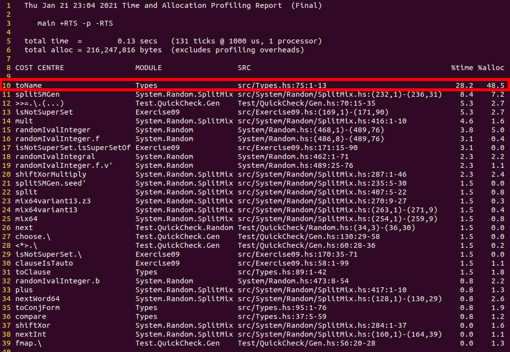
As you can see, 28.2% of the runtime was spent on the function toName.
Now, perhaps to your surprise, toName is simply defined as follows:
toName :: String -> Int
toName = read
where read is the very standard function to transform a String to some value a provided that Read a.
That seems quite strange – how can this standard library function be so slow?
The problem is very well described in this StackOverflow discussion:
read is doing quite a bit more than one expects, e.g. (read "(- 124)" :: Int) = 124.
It is more a parser than a simple character to digit converter.
Luckily, StackOverflow also holds a solution: we can use the more efficient readInt from bytestring:
toName = fst . fromJust . LC.readInt . LC.packAnother bottleneck of most submissions was subsumption checking. Checking subset-relationships for each clause is very expensive. Some students realised this and added some pre-conditions before actually checking for subset-equality:
- if \(|C|>|C'|\) then \(C\not\subseteq C'\)
- if \[\bigl|\{l\in C\mid l\text{ is positive}\}\bigr|>|\{l\in C'\mid l\text{ is positive}\}|\] then \(C\not\subseteq C'\)
- if \[\bigl|\{l\in C\mid l\text{ is negative}\}\bigr|>|\{l\in C'\mid l\text{ is negative}\}|\] then \(C\not\subseteq C'\)
Further optimisations will need some more ingenuity. We’ll discuss them further below. But now let’s have a look at the results!
Run 1
Parameters
| Generator | Timeout [seconds] | #Test Cases | QC Seed | Freq. Pos Vars | Freq. Neg Vars | Max. Var | Max. Clause Size | Max. #Clauses |
|---|---|---|---|---|---|---|---|---|
genEConjForm1(14% refutations) |
20 | 100 | 1337 | 1 | 1 | 5 | 8 | 20 |
Results
Interestingly enough, two so far innocent submissions commited proof-crime, i.e. submitted a faulty proof. The judge of logic speaks: Schuldig! 👨⚖️ Herr Brandt and Herr Krayer are banned for this test suite.
| Rank | Name | Time [seconds] |
|---|---|---|
| 1. | MC Jr | 0.01 |
| 1. | Christiane Kobalt | 0.01 |
| 1. | Florian Hübler | 0.02 |
| 1. | Benjamin Defant | 0.02 |
| 1. | Jalil Salamé Messina | 0.02 |
| 1. | Julian Pritzi | 0.02 |
| 1. | Luis Bahners | 0.02 |
| 1. | Sophia Knapp | 0.03 |
| 1. | Robert Imschweiler | 0.03 |
| 1. | Tobias Markus | 0.03 |
| 1. | Vitus Hofmeier | 0.04 |
| 1. | Niclas Schwalbe | 0.04 |
| 1. | Jakob Florian Goes | 0.05 |
| 1. | Aaron Tacke | 0.09 |
| 15. | Markus Englberger | 0.18 |
| 15. | Simon Longhao Ouyang | 0.19 |
| 15. | Jonas Benjamin Goos | 0.21 |
| 18. | Dominik Weinzierl | 0.50 |
| 18. | JiWoo Hwang | 0.57 |
| 20. | Jakub Stastny | 7.88 |
| 21. | Felix Zehetbauer | TIMEOUT |
| 21. | Flavio Principato | TIMEOUT |
| 21. | Cara Dickmann | TIMEOUT |
| 21. | Eddie Groh | TIMEOUT |
| 21. | Niklas Lohmann | TIMEOUT |
| 21. | Christoph Starnecker | TIMEOUT |
| 21. | Florian Schmidt | TIMEOUT |
| 21. | Max Schröder | TIMEOUT |
| 21. | Felix Brandis | TIMEOUT |
| X | Björn Brandt | FAULTY PROOF |
| X | Felix Krayer | FAULTY PROOF |
Run 2
Parameters
| Generator | Timeout [seconds] | #Test Cases | QC Seed | Freq. Pos Vars | Freq. Neg Vars | Max. Var | Max. Clause Size | Max. #Clauses |
|---|---|---|---|---|---|---|---|---|
genEConjForm1(71% refutations) |
20 | 100 | 1337 | 1 | 1 | 5 | 8 | 100 |
Results
Every student passed this round 🎉
| Rank | Name | Time [seconds] |
|---|---|---|
| 1. | Julian Pritzi | 0.04 |
| 1. | MC Jr | 0.04 |
| 1. | Christiane Kobalt | 0.04 |
| 1. | Tobias Markus | 0.04 |
| 1. | Vitus Hofmeier | 0.04 |
| 1. | Luis Bahners | 0.04 |
| 1. | Florian Hübler | 0.05 |
| 1. | Jalil Salamé Messina | 0.07 |
| 1. | Robert Imschweiler | 0.09 |
| 1. | Benjamin Defant | 0.10 |
| 11. | Markus Englberger | 0.13 |
| 11. | Sophia Knapp | 0.13 |
| 11. | Niclas Schwalbe | 0.20 |
| 11. | Simon Longhao Ouyang | 0.22 |
| 15. | Jonas Benjamin Goos | 0.36 |
| 16. | Dominik Weinzierl | 0.63 |
| 17. | Aaron Tacke | 1.14 |
| 18. | Jakob Florian Goes | 3.03 |
| 18. | Jakub Stastny | 3.05 |
| 20. | JiWoo Hwang | 5.61 |
Run 3
Parameters
| Generator | Timeout [seconds] | #Test Cases | QC Seed | Freq. Pos Vars | Freq. Neg Vars | Max. Var | Max. Clause Size | Max. #Clauses |
|---|---|---|---|---|---|---|---|---|
genEConjForm1(84% refutations) |
20 | 100 | 1337 | 1 | 1 | 10 | 8 | 200 |
Results
Some provers got pushed beyond their capabilities…
| Rank | Name | Time [seconds] |
|---|---|---|
| 1. | MC Jr | 0.08 |
| 1. | Luis Bahners | 0.10 |
| 3. | Christiane Kobalt | 0.15 |
| 3. | Julian Pritzi | 0.15 |
| 3. | Florian Hübler | 0.16 |
| 3. | Tobias Markus | 0.17 |
| 7. | Benjamin Defant | 0.21 |
| 7. | Robert Imschweiler | 0.23 |
| 9. | Jakob Florian Goes | 0.39 |
| 10. | Sophia Knapp | 0.50 |
| 11. | Niclas Schwalbe | 1.39 |
| 12. | Aaron Tacke | 10.50 |
| 13. | Jonas Benjamin Goos | 11.28 |
| 14. | Jalil Salamé Messina | 16.66 |
| 15. | Dominik Weinzierl | TIMEOUT |
| 15. | JiWoo Hwang | TIMEOUT |
| 15. | Jakub Stastny | TIMEOUT |
| 15. | Simon Longhao Ouyang | TIMEOUT |
| 15. | Markus Englberger | TIMEOUT |
| 15. | Vitus Hofmeier | TIMEOUT |
Run 4
Parameters
| Generator | Timeout [seconds] | #Test Cases | QC Seed | Freq. Pos Vars | Freq. Neg Vars | Max. Var | Max. Clause Size | Max. #Clauses |
|---|---|---|---|---|---|---|---|---|
genEConjForm1(99% refutations) |
20 | 100 | 1337 | 2 | 1 | 20 | 10 | 2000 |
Results
…but the number of clauses relentlessly increases.
| Rank | Name | Time [seconds] |
|---|---|---|
| 1. | Jakob Florian Goes | 1.82 |
| 1. | MC Jr | 1.87 |
| 3. | Tobias Markus | 2.26 |
| 3. | Jalil Salamé Messina | 2.33 |
| 5. | Julian Pritzi | 2.58 |
| 6. | Benjamin Defant | 2.91 |
| 7. | Luis Bahners | 2.85 |
| 8. | Florian Hübler | 3.13 |
| 9. | Christiane Kobalt | 3.67 |
| 10. | Robert Imschweiler | 4.10 |
| 11. | Jonas Benjamin Goos | 9.25 |
| 12. | Aaron Tacke | TIMEOUT |
| 12. | Sophia Knapp | TIMEOUT |
| 12. | Niclas Schwalbe | TIMEOUT |
Run 5
Parameters
| Generator | Timeout [seconds] | #Test Cases | QC Seed | Freq. Pos Vars | Freq. Neg Vars | Max. Var | Max. Clause Size | Max. #Clauses |
|---|---|---|---|---|---|---|---|---|
genEConjForm1(95% refutations) |
20 | 100 | 1337 | 1 | 1 | 40 | 25 | 2500 |
Results
Until at some point…
| Rank | Name | Time [seconds] |
|---|---|---|
| 1. | MC Jr | 0.28 |
| 2. | Luis Bahners | 0.68 |
| 3. | Robert Imschweiler | 0.85 |
| 4. | Tobias Markus | 1.06 |
| 4. | Christiane Kobalt | 1.15 |
| 6. | Florian Hübler | 14.68 |
| 7. | Jonas Benjamin Goos | TIMEOUT |
| 7. | Benjamin Defant | TIMEOUT |
| 7. | Jalil Salamé Messina | TIMEOUT |
| 7. | Jakob Florian Goes | TIMEOUT |
| 7. | Julian Pritzi | TIMEOUT |
Run 6
Parameters
| Generator | Timeout [seconds] | #Test Cases | QC Seed | Freq. Pos Vars | Freq. Neg Vars | Max. Var | Max. Clause Size | Max. #Clauses |
|---|---|---|---|---|---|---|---|---|
genEConjForm1(80% refutations) |
20 | 10 | 1337 | 1 | 1 | 100 | 50 | 5000 |
Results
…only one prover can survive.
| Rank | Name | Time [seconds] |
|---|---|---|
| 1. | MC Jr | 0.58 |
| 2. | Florian Hübler | TIMEOUT |
| 2. | Christiane Kobalt | TIMEOUT |
| 2. | Robert Imschweiler | TIMEOUT |
| 2. | Tobias Markus | TIMEOUT |
| 2. | Luis Bahners | TIMEOUT |
Run 7
Parameters
| Generator | Timeout [seconds] | #Test Cases | QC Seed | Freq. Pos Vars | Freq. Neg Vars | Max. Var | Max. Clause Size | Max. #Clauses |
|---|---|---|---|---|---|---|---|---|
genEConjForm1(100% refutations) |
20 | 5 | 1337 | 1 | 1 | 100 | 30 | 300.000 |
Results
For the curious, even formulas with 300.000 clauses can be solved in reasonable time.
| Name | Time [seconds] |
|---|---|
| MC Jr | 15.21 |
Scores
Alright, let’s discuss our champions’ solutions. We already talked a lot about Herr Imschweiler and the beauty and simplicity of Frau Kobalt’s submission. What about Herr Hübler, Markus, and Bahners?
Herr Hübler uses an interesting heuristic that limits the size of created clauses. Only if no refutation can be found below that limit, it will be increased to salvage completeness. In fact, Herr Hübler does not use the clauses’ size but number of distinct variables. Though to the MC Jr, that just overcomplicates things as variables should be unique in clauses anyway, unless the clause is tautological, in which case it can be removed all together… But let the artist speak for himself:
{-
The basics of my algorithm are the same, some specifications:
preOpt: Removes duplicates inside clauses
        Removes Tautos
        Removes Clauses which are implied by other clauses
        Calculated the maximum number of unique variables (Pos a =/= Neg a) in a Clause
selClause:  Selects the clause with the least number of unique Variables

The Bigger changes I made include:
When new Clauses are added by resolving, they are only added if
    - They are not already implied by already existing clauses
    - They are no tautos
    - They have less unique Variables than maxWeight

The idea of maxWeight is, to prevent the creation of huge clauses as they will most likely just grow bigger
Due to maxWeight we cannot guarantee anymore that a saturated set of clauses can be fullfilled hence we have to check that
and if it is not fullfilled we increase the maxWeight and go again.

For very large inputs maxWeight could be decreased to (floor $ maxWeight / 2) if the clause sizes have a high variance
    Nevermind, I changed it to maxLength / 2 now incase there is one long ass clause while all the others are smaller
    Maybe average * 1.5 might be even better but idc anymore, this is good enough -}
Herr Markus maintains a map from literals to keys of clauses that contain the given literal, which he calls
OccursMap. This map can be used to efficiently retrieve candidate clauses when doing subsumption checks: for each literal in a given clause, retrieve all clauses containing the literal and then intersect all these sets to obtain the exact set of subsumed clauses.At least the MC Jr thinks that’s what he does; his code is rather cryptic and without comments 🙊Update 25.01: Herr Markus confirmed by e-mail that this in fact is what he is doing 📧Herr Bahners, though winning this round, is in some sense the most boring solution: he very strictly followed the exercise sheet’s pseudo-algorithm, and besides that, just added whatever has been suggested so far. No surprises, no cyrptic functions. His code is pure, clean, beautiful, efficient. A boring masterpiece! 👨🎨🖼 It seems to be a pattern that clarity outperforms overengineering in this competition.
| Rank | Name | Score |
|---|---|---|
| 1. | Luis Bahners | 30*3 |
| 2. | Robert Imschweiler | 29*3 |
| 3. | Tobias Markus | 27.5*3 |
| 3. | Christiane Kobalt | 27.5*3 |
| 5. | Florian Hübler | 26*3 |
| 6. | Jakob Florian Goes | 25*3 |
| 7. | Jalil Salamé Messina | 24*3 |
| 8. | Julian Pritzi | 23*3 |
| 9. | Benjamin Defant | 22*3 |
| 10. | Jonas Benjamin Goos | 21*3 |
| 11. | Sophia Knapp | 20*3 |
| 12. | Niclas Schwalbe | 19*3 |
| 13. | Aaron Tacke | 18*3 |
| 14. | Vitus Hofmeier | 17*3 |
| 15. | Markus Englberger | 15.5*3 |
| 15. | Simon Longhao Ouyang | 15.5*3 |
| 17. | Dominik Weinzierl | 14*3 |
| 18. | Jakub Stastny | 13*3 |
| 19. | JiWoo Hwang | 12*3 |
| 20. | Felix Zehetbauer | 7*3 |
| 20. | Flavio Principato | 7*3 |
| 20. | Cara Dickmann | 7*3 |
| 20. | Eddie Groh | 7*3 |
| 20. | Niklas Lohmann | 7*3 |
| 20. | Christoph Starnecker | 7*3 |
| 20. | Florian Schmidt | 7*3 |
| 20. | Max Schröder | 7*3 |
| 20. | Felix Brandis | 7*3 |
| X | Björn Brandt | 0 |
| X | Felix Krayer | 0 |
Test 4: Pigeonhole ❗
As a bonus round, it is tradition that the MC Jr tortures all poor solvers using the pigeonhole formula.
The pigeonhole formula tries to put \(n+1\) pigeons into \(n\) holes such that each hole contains at most 1 pigeon. Obviously, such an assignment is impossible. However, naive resolution provers like ours have an exponential time best case complexity for these formulas.
The pigeonhole formula can be modelled as follows:
\[ \begin{align} &\Bigl\{\{x_{i,1},\dotsc,x_{i,n}\} \mid 1\leq i\leq n+1 \Bigr\}\\ \cup\quad&\Bigl\{\{\lnot x_{i,k}, \lnot x_{j,k}\} \mid 1\leq i \leq n+1,\, 1 \leq k \leq n,\, i\neq k\Bigr\} \end{align} \] The first set ensures that each pigeon is in at least one hole, the second one that there cannot be two pigeons in the same hole. It’s time for exponential blowups! 💣
Run 1
Parameters
| Generator | Timeout [seconds] | #Test Cases | #Pigeons (\(n+1\)) |
|---|---|---|---|
genEConjFormPigeonhole |
20 | 1 | 3 |
Results
Besides those 4 provers that apparently got so scared they suddenly returned a faulty proof, 3 pigeons and 2 holes seem to be no problem for all candidates.
| Rank | Name | Time [seconds] |
|---|---|---|
| 1. | Sophia Knapp | 0.00 |
| 1. | MC Jr | 0.00 |
| 1. | Flavio Principato | 0.00 |
| 1. | Florian Hübler | 0.00 |
| 1. | Dominik Weinzierl | 0.00 |
| 1. | Cara Dickmann | 0.00 |
| 1. | Eddie Groh | 0.00 |
| 1. | Benjamin Defant | 0.00 |
| 1. | Jalil Salamé Messina | 0.00 |
| 1. | Jakob Florian Goes | 0.00 |
| 1. | Jakub Stastny | 0.00 |
| 1. | Christiane Kobalt | 0.00 |
| 1. | Julian Pritzi | 0.00 |
| 1. | Simon Longhao Ouyang | 0.00 |
| 1. | Markus Englberger | 0.00 |
| 1. | Robert Imschweiler | 0.00 |
| 1. | Tobias Markus | 0.00 |
| 1. | Christoph Starnecker | 0.00 |
| 1. | Aaron Tacke | 0.00 |
| 1. | Felix Zehetbauer | 0.00 |
| 1. | Vitus Hofmeier | 0.00 |
| 1. | Niclas Schwalbe | 0.00 |
| 1. | Luis Bahners | 0.00 |
| 1. | Felix Brandis | 0.00 |
| 1. | Jonas Benjamin Goos | 0.01 |
| 1. | JiWoo Hwang | 0.01 |
| 1. | Niklas Lohmann | 0.01 |
| X | Björn Brandt | FAULTY PROOF |
| X | Felix Krayer | FAULTY PROOF |
| X | Florian Schmidt | FAULTY PROOF |
| X | Max Schröder | FAULTY PROOF |
Run 2
Parameters
| Generator | Timeout [seconds] | #Test Cases | #Pigeons (\(n+1\)) |
|---|---|---|---|
genEConjFormPigeonhole |
20 | 1 | 4 |
Results
Now if we ask to put 4 pigeons into three holes, some provers are already hopelessly overwhelmed.
| Rank | Name | Time [seconds] |
|---|---|---|
| 1. | MC Jr | 0.00 |
| 1. | Christoph Starnecker | 0.00 |
| 1. | Luis Bahners | 0.00 |
| 1. | Flavio Principato | 0.01 |
| 1. | Florian Hübler | 0.01 |
| 1. | Robert Imschweiler | 0.01 |
| 1. | Niclas Schwalbe | 0.01 |
| 1. | Felix Zehetbauer | 0.01 |
| 1. | Felix Brandis | 0.01 |
| 1. | Christiane Kobalt | 0.02 |
| 1. | Tobias Markus | 0.02 |
| 1. | Sophia Knapp | 0.03 |
| 1. | Cara Dickmann | 0.03 |
| 1. | Julian Pritzi | 0.03 |
| 1. | Benjamin Defant | 0.04 |
| 1. | Aaron Tacke | 0.04 |
| 1. | Jakub Stastny | 0.05 |
| 1. | Vitus Hofmeier | 0.06 |
| 19. | Jakob Florian Goes | 0.25 |
| 20. | Eddie Groh | 0.47 |
| 21. | Jonas Benjamin Goos | 3.92 |
| 22. | Jalil Salamé Messina | 11.26 |
| 23. | JiWoo Hwang | 12.28 |
| 24. | Dominik Weinzierl | TIMEOUT |
| 24. | Simon Longhao Ouyang | TIMEOUT |
| 24. | Markus Englberger | TIMEOUT |
| 24. | Niklas Lohmann | TIMEOUT |
Run 3
Parameters
| Generator | Timeout [seconds] | #Test Cases | #Pigeons (\(n+1\)) |
|---|---|---|---|
genEConjFormPigeonhole |
20 | 1 | 5 |
Results
More pigeons are to come and fewer provers to stay!
| Rank | Name | Time [seconds] |
|---|---|---|
| 1. | MC Jr | 0.01 |
| 2. | Luis Bahners | 0.36 |
| 3. | Tobias Markus | 3.02 |
| 4. | Florian Hübler | 3.16 |
| 4. | Robert Imschweiler | 3.17 |
| 6. | Christiane Kobalt | 8.73 |
| 7. | Niclas Schwalbe | 12.44 |
| 8. | Christoph Starnecker | 14.82 |
| 9. | Sophia Knapp | 16.44 |
| 10. | Flavio Principato | TIMEOUT |
| 10. | Felix Zehetbauer | TIMEOUT |
| 10. | Jonas Benjamin Goos | TIMEOUT |
| 10. | Cara Dickmann | TIMEOUT |
| 10. | Eddie Groh | TIMEOUT |
| 10. | Benjamin Defant | TIMEOUT |
| 10. | Jalil Salamé Messina | TIMEOUT |
| 10. | JiWoo Hwang | TIMEOUT |
| 10. | Jakob Florian Goes | TIMEOUT |
| 10. | Jakub Stastny | TIMEOUT |
| 10. | Julian Pritzi | TIMEOUT |
| 10. | Aaron Tacke | TIMEOUT |
| 10. | Vitus Hofmeier | TIMEOUT |
| 10. | Felix Brandis | TIMEOUT |
Run 4
Parameters
| Generator | Timeout [seconds] | #Test Cases | #Pigeons (\(n+1\)) |
|---|---|---|---|
genEConjFormPigeonhole |
40 | 1 | 6 |
Results
Can we put 6 pigeons into 5 holes? Let’s increase the timeout to 40 seconds to let our provers think about it more thoroughly.
| Rank | Name | Time [seconds] |
|---|---|---|
| 1. | MC Jr | 0.01 |
| 2. | Luis Bahners | 1.04 |
| 3. | Robert Imschweiler | 17.76 |
| 4. | Christiane Kobalt | 37.52 |
| 5. | Sophia Knapp | TIMEOUT |
| 5. | Florian Hübler | TIMEOUT |
| 5. | Tobias Markus | TIMEOUT |
| 5. | Christoph Starnecker | TIMEOUT |
| 5. | Niclas Schwalbe | TIMEOUT |
Run 5
Parameters
| Generator | Timeout [seconds] | #Test Cases | #Pigeons (\(n+1\)) |
|---|---|---|---|
genEConjFormPigeonhole |
40 | 1 | 7 |
Results
And TIMEOUT! 6 pigeons and not a single more is what this year’s
provers were able to handle.
The MC Jr’s prover is doing a bit better, solving the case for 8 pigeons
in about 8 seconds.
But once the 9th bird joins in, also his prover throws the towel 🤷
| Rank | Name | Time [seconds] |
|---|---|---|
| 1. | MC Jr | 0.15 |
| 2. | Luis Bahners | TIMEOUT |
| 2. | Robert Imschweiler | TIMEOUT |
| 2. | Christiane Kobalt | TIMEOUT |
Scores
Once more, we find the usual suspects on the top of the hill.
| Rank | Name | Score |
|---|---|---|
| 1. | Luis Bahners | 30 |
| 2. | Robert Imschweiler | 29 |
| 3. | Christiane Kobalt | 28 |
| 4. | Tobias Markus | 27 |
| 5. | Florian Hübler | 26 |
| 6. | Niclas Schwalbe | 25 |
| 7. | Christoph Starnecker | 24 |
| 8. | Sophia Knapp | 23 |
| 9. | Flavio Principato | 18 |
| 9. | Felix Zehetbauer | 18 |
| 9. | Felix Brandis | 18 |
| 9. | Cara Dickmann | 18 |
| 9. | Julian Pritzi | 18 |
| 9. | Benjamin Defant | 18 |
| 9. | Aaron Tacke | 18 |
| 9. | Jakub Stastny | 18 |
| 9. | Vitus Hofmeier | 18 |
| 18. | Jakob Florian Goes | 13 |
| 19. | Eddie Groh | 12 |
| 20. | Jonas Benjamin Goos | 11 |
| 21. | Jalil Salamé Messina | 10 |
| 22. | JiWoo Hwang | 9 |
| 23. | Dominik Weinzierl | 7 |
| 23. | Simon Longhao Ouyang | 7 |
| 23. | Markus Englberger | 7 |
| 23. | Niklas Lohmann | 7 |
| X | Björn Brandt | 0 |
| X | Felix Krayer | 0 |
| X | Florian Schmidt | 0 |
| X | Max Schröder | 0 |
The MC Jr’s Solution 🤓
Before we announce the winner, the MC Jr wants to reveal his final few tricks 🃏 Once you want to go beyond what we covered so far, your best friends are research papers and lecture notes. It’s time for some theory! 📚
Efficient Subsumption Checking
The heuristics described above are nice to get started, but very limited. It is terribly inefficient to traverse the whole set of clauses whenever we want to check for subsumption. Think about hundreds of thousands of clauses!
There are various ways of improving this state of affairs. One very elegant and simple idea is Feature Vector Indexing, invented by Stephan Schulz for the E theorem prover some time ago at TUM! Excellent.
In the case of propositional logic, we can build a feature vector trie whose edges indicate whether the next largest literal is contained in a given set of clauses. For example, given the formulas
c1 = [¬6, ¬1], c2 = [¬5, 1], c3 = [¬5, 2]we can buld the following feature vector trie:
    {c1,c2,c3}
        /\
     -6/  \
      /    \
    {c1}  {c2,c3}
  -1|     -5|
    |       |
   {c1} {c2,c3}
         1|   \
          |    \
        {c2}    {c3}
                2|
                 |
                {c3}
Removing all subsumed clauses of the set or checking whether a clause is subsumed now becomes as simple as traversing (and updating) the trie! You can checkout the MC Jr’s implementation here.
Ordered Resolution With Selection
The following optimisations takes more than algorithmic intuition: If one carefully checks the proof of the model existence theorem, which the MC Jr referred to on the exercise sheet, one can see that the algorithm stays complete even if we
- (ordered resolution) only resolve maximal literals in each clause (with respect to the order as was given in the template), and
- (selection) prefer negative literals by an arbitrary selection strategy.
Funnily enough, the linked source on the exercise sheet has been taken offline by now. Maybe too many curious students DDoSed the website!? 🌩 In any case, you can read about this insight in the Automated Reasoning lecture notes of the MPI-Saarland, Section 3.12. In fact, this insight even generalises to first-order logic resolution!
Summa summarum, the above allows us to skip many, many resolution steps. As a literal selection strategy, the MC Jr decided to simply select the smallest, negative literal of a clause.
Example 1:
Given the clauses c1 = [-1] and c2 = [1,2], standard resolution derives the clause [2].
Ordered resolution, on the other hand, derives no clause as 1 is not maximal in c2.
Example 2:
Given the clauses c1 = [-2] and c2 = [-1,2],
ordered resolution derives the clause [-1].
Ordered resolution with selection, on the other hand, derives no clause as the literal -1 is selected in c2.
Caching Data
As a final optimisation step, the MC Jr realised – once again, thanks to the profiler – that searching for the minimal literal of a clause over and over again is not a particularly good idea.
So as a final optimisation, he added an additional Data field to his clauses where he caches the minimal literal of a given clause.
More generally, it is always a good idea to cache non-trivial, re-occuring computations in such data fields.
Conclusion
There were many sophisticated submissions! The MC Jr has to tip his hat – he is very proud of you 🎩 Here are some takeaways for the future. Remember these words:
- Never trust unverified code: many provers tried to trick us with faulty proofs! 🤨
- Efficient data structures are extremely important 👨💻
- Clean and modular code often results in more efficient code ✨
- Those who don’t subsume, will be subsumed
- Profiling reveals many weaknesses 🔍
- To be practical, you need to think theoretical! 👩🏫
- Logic can be theoretical, practical, and, most importantly, fun!
The MC Jr dearly hopes you enjoyed this week’s logic special 😊 Maybe some of you will come back for more at the Q.E.D. chair. We will offer a logic course, a functional data structures course, and a functional programming seminar next semester. See you there!
Final Scores Week 8
Here it is: the prestigious ranking of logic connoisseurs 👏👏👏
| Rank | Name | Points | Score |
|---|---|---|---|
| 🥇 | Luis Bahners | 30 | 178.5 |
| 🥈 | Robert Imschweiler | 29 | 167.5 |
| 🥉 | Tobias Markus | 28 | 149.0 |
| 4. | Christiane Kobalt | 27 | 148.0 |
| 5. | Florian Hübler | 26 | 145.5 |
| 6. | Julian Pritzi | 25 | 140.5 |
| 7. | Jalil Salamé Messina | 24 | 133.0 |
| 8. | Benjamin Defant | 23 | 130.0 |
| 9. | Sophia Knapp | 22 | 119.0 |
| 10. | Niclas Schwalbe | 21 | 117.0 |
| 11. | Jakob Florian Goes | 20 | 116.5 |
| 12. | Vitus Hofmeier | 19 | 102.0 |
| 13. | Jonas Benjamin Goos | 18 | 101.0 |
| 14. | Aaron Tacke | 17 | 100.5 |
| 15. | Simon Longhao Ouyang | 16 | 84.0 |
| 16. | Jakub Stastny | 15 | 81.0 |
| 17. | Dominik Weinzierl | 14 | 79.5 |
| 17. | Markus Englberger | 14 | 79.5 |
| 19. | Flavio Principato | 12 | 71.5 |
| 20. | Felix Zehetbauer | 11 | 65.0 |
| 21. | Christoph Starnecker | 10 | 62.5 |
| 21. | JiWoo Hwang | 10 | 62.5 |
| 23. | Felix Brandis | 8 | 56.5 |
| 23. | Cara Dickmann | 8 | 56.5 |
| 25. | Niklas Lohmann | 6 | 53.0 |
| 26. | Eddie Groh | 5 | 50.5 |
| 27. | Florian Schmidt | 4 | 38.5 |
| 27. | Max Schröder | 4 | 38.5 |
| 29. | Felix Krayer | 2 | 23.0 |
| 30. | Björn Brandt | 1 | 22.0 |
FPV-Programming Contest
This is not a normal Wettbewerbs-entry (sad noises in the distance), but just a short recap of our first-ever FPV Programming Contest (10.02.2021).
The contest was very much in the spirit of an ICPC:
teams of 2–3 students tried to solve as many programming puzzles as possible in a 4 hour timeslot.
All problems were (more or less) creatively written by our tutors, the MC Jr Jr, and the MC Jr (the author of this short blog entry).
In contrast to a normal ICPC, however, we only allowed submissions in the most beautiful of languages taught at TUM, i.e. Haskell™,
submitted via Artemis™;
and in contrast to homework submissions on Artemis, participants did not get any feedback other than Wrong, Correct, or Timeout.
Moreover, teams were allowed to work on problems in parallel and use the Internet, including copying of source code if cited appropriately.
In all honesty, the MCs and their tutor team were a bit worried that participation might be low,
but the FPV students cohort proved them wrong:
27 brave teams joined the competition 👏
This particularly put our tutors – Marco and Korbi – responsible for the contest website under great pressure.
Behind the scenes, both the problems setup and website were ready just moments before the start of the contest.
But even though our tutors commited the cardinal sin of using Python instead of Haskell to program the backend server,
nothing went wrong and the website looks magnificent.
Indeed, the only thing that failed us is the team naming feature of Artemis:
as 2 teams sadly had to experience, having a leading digit in one’s team name
leads to internal server errors on Artemis.
Bug reported! 🐞
Team 114514 swiftly got renamed to artemishatesleadingdigits
and team 0xb5ce2e78bbce to teamtechproblem.
Now as for the contest, we decided to freeze the scoreboard after 3 hours and unfreeze it once
all problem solutions were discussed following the 4 hours programming time slot.
However, our winning team – haskellhackers – spoilt the fun by finishing all exercises in an insane 2 1/2 hours speedrun.
How dare they ruining our exciting idea! 😜
This victory came a bit as a surprise because some other teams had a better start.
In particular our Polish team szczebrzeszyńskadrużyna started like a rocket 🚀 finishing 4/7 problems in just 30 minutes.
The MCs were already practising their Polish in order to somehow stutter the expected winner’s team name correctly!
Luckily, we were spared that humiliation 😅
Even though the winning team was already fixed, the contest remained thrilling till the very end.
Most teams were part of a close head-to-head race,
the final results only becoming clear once the scoreboard unfroze again.
To build up tension, we of course first discussed and revealed the problem solutions on BBB before unfreezing the scoreboard.
You can find the set of slides and solution approaches here.
As it turned out during our discussions, some teams managed to pass some tests with non-optimal algorithms
and data structures.
In particular, team ['g','h','z','i'] (joke shamelessly stolen and adapted) abused lists as sets, maps, lookup tables, etc.
Seems like the MCs were a bit too generous when setting the time limits of the tests.
In a poll on BBB, participants almost unanimously agreed on that contests like this are a lot of fun. We are very happy that you enjoyed it! 😊 We hope to make the platform available to other lectures in the future. Until then, we also suggest you to join the official ICPC events hosted at TUM. Have a look at their website. Moreover, we can recommend the fun Practical Course – Algorithms for Programming Contests.
Finally, here are the final results including the awarded Wettbewerb points of the contest. You can find the detailed results on the contest website. See you on Friday, 12.02.2021 for our Semester Closing event!
Final Scores FPV-Programming Contest
| Rank | Team | Name #1 | Name #2 | Name #3 | Score |
|---|---|---|---|---|---|
| 🥇 | haskellhackers | Rafael Brandmaier | Simon Weigl | Nils Cremer | 30 |
| 🥈 | ghzi | Robert Imschweiler | Vitus Hofmeier | Felix Zehetbauer | 29 |
| 🥉 | maol | Max Lang | Oliver Lemke | Alisa Parashchenko | 28 |
| 4. | gbs2021 | Tony Wang | Tobias Lindenbauer | Rebecca Ghidini | 27 |
| 5. | ninjaturtles | Benjamin Defant | Fabian Wenz | Florian Hübler | 26 |
| 6. | artemishatesleadingdigits (114514) | Xuemei Zhang | Peilai Yu | Simon Longhao Ouyang | 25 |
| 7. | recursivenomads | Alexey Glushik | Aleksandr Mavrichev | Egor Spirin | 24 |
| 8. | pat | Thomas Sedlmeyr | Aaron Tacke | Philip Haitzer | 23 |
| 9. | teamtechproblem (0xb5ce2e78bbce) | Malte Schmitz | Olha Dolhova | Philipp Wittmann | 22 |
| 10. | mikado | Noah Dormann | Simon Kammermeier | 21 | |
| 11. | szczebrzeszyńskadrużyna | Alejandro Tang Ching | Patryk Morawski | 20 | |
| 12. | spaghettichefs9000 | Sophia Knapp | Philipp Sanwald | Jalil Salamé Messina | 19 |
| 13. | teamhaskel1337 | Li-Ming Bao | Tim Hertel | Cedric Theato | 18 |
| 14. | syzygy | Paul Hofmeier | Tobias Markus | Christiane Kobalt | 17 |
| 15. | funktionalefeinis | Simon Pannek | Christoph Rotte | Severin Schmidmeier | 16 |
| 16. | functional0programators | Julian Sikora | Matthias Ritzenhoff | JiWoo Hwang | 15 |
| 17. | l3bkuch3n | Denitsa Keranova | David Alkier | Thilo Linke | 14 |
| 18. | turtlemasters | Christian Zimmerer | Krishna Mavani | 13 | |
| 19. | foobar | Marc Maximilian Fett | Adrian Reuter | Markus Englberger | 12 |
| 20. | tumbum | Adam Nanouche | Philipp Eisermann | Simon Karan Guayana | 11 |
| 21. | antitaktik | Felix Schnabel | Arcangelo Capozzolo | 10 | |
| 22. | qed | Elias Panner | Tobias Schamel | 9 | |
| 23. | formfollowsfunction | Alexander Stephan | Luisa Ortner | Prakriti Sabharwal | 8 |
| 24. | lemmahaveagoodtime | Leonardo Maglanoc | Julia Spindler | 7 | |
| 25. | schwarzinformatik | Tim Ortel | Stefanie Manger | 6 | |
| 26. | munichesports | Marco Ring | Jan Nicolas Weßeling | Robin Franke | 5 |
| 27. | aninvisibleparticipant | Jonas Ballweg | Sohrab Tawana | Daniel Schwermann | 4 |
Schönheitswettbewerb & Semester Closing
This, we are afraid to say, is our final blog entry (presumably, for a long time). We want to thank all of you for your enthusiasm and wonderful submissions. Every year, our students exceed all expectations; this year being no exception. Your creativity, diligence and enthusiasm is amazing. Keep it up!
This year was a bit special as we tried many new things like workshops offered by people from industry,
the FPV-programming contest, creative homeworks designed by tutors, 🗣 FPV & Chill 🍻, etc.
At this point, we once again want to thank all of our wonderful tutors for making this possible.
Thanks to:
Paul Bachmann,
Benjamin Bott,
Omar Eldeeb,
Alexey Gavryushin,
Bilel Ghorbel,
Jakob Gottfriedsen,
Patrick Großmann,
Philipp Hagenlocher,
Simon Hanssen,
Marco Haucke,
Yi He,
Jonas Hübotter,
Kira Nickel,
Alexandrina Panfil,
Mete Polat,
Justus Polzin,
Fabian Pröbstle,
Simon Stieger,
Mira Trouvain,
Korbinian Weidinger,
Thomas Wimmer, and
Leon Zamel
We hope you all enjoyed the award ceremony on Friday evening (12.02). As mentioned there, we now updated the semester ranking and will contact all award winners soon by e-mail. For those of you that missed it, here are the ceremony slides and the 11 glorious submissions of the FPV-Schönheitswettbewerb 2021, ranked by the Q.E.D. Chair:
Update 14.02: The points for Herr Hübler on the slides are wrong: he did not score 197 but 226 points!
Update 15.02: Added submission by Herr Ouyang.
Glitch – by Herr Ouyang
For spot 11, Herr Ouyang submitted not so much a piece of art but a piece to destroy art. His glitch tool allows you to take your favourite painting and “ruining” it with glitches. Well actually, lovers of Glitch Art would not say “ruin” but rather “enhance” it. In any case, the Wettbewerb is open to (almost) any art form. Here are some simple examples submitted by our Haskell artist:


Loss – by Herr Brandt
Also on spot 11, we find a submission that left the ranking committee in great confusion. Due to that, it might actually have been the most artsy of all submissions. Luckily, at our Semester Closing Party, the artist himself had the chance to explain the meaning of the image. And of course, it being the year 2021, nothing but a meme could be the explanation. As his peers realised, the fourth panel is sadly missing. Nevertheless, a subtle piece of art!
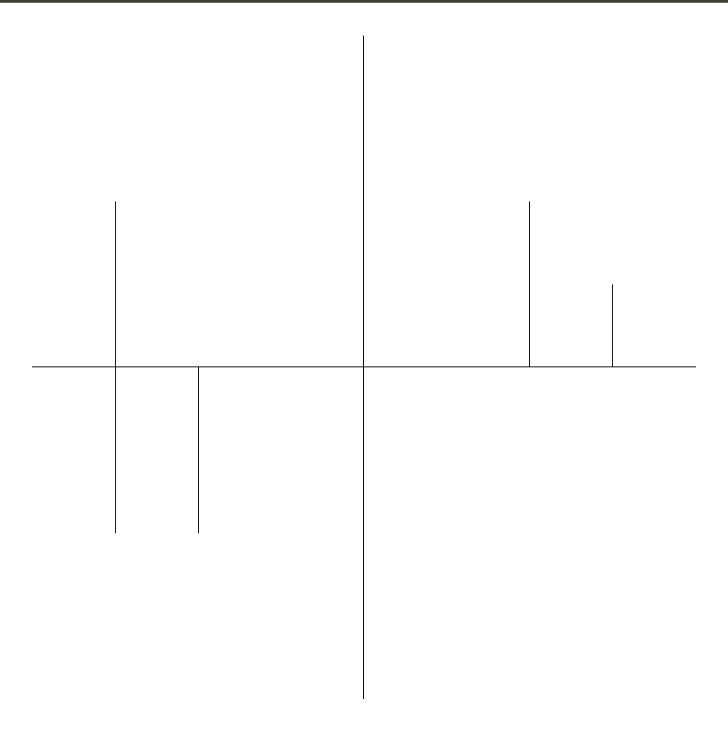
Frozen Snowflakes
On spot 8-10, we find 3 pretty snowflake submissions, handturtle-drawn by our artists.
Enjoy the freezing winter atmosphere ❄❄❄
Herr Brandmaier
In Herr Braindmaier’s submission, we find a whole army of snowflakes.

Herr Principato
Herr Principato, to the MCs’ great amusement, besides his snowflakes, also submitted an accompanying meme:


Herr Defant
Finally, Herr Defant not only made his turtle draw a very colourful snowflake, but also a Sierpiński triangle.

Moving Snowflakes – by Herr Hofmeier
There indeed have been many snowflake submissions, but our artist on spot 6 (shared with Herr Zehetbauer) went a step further than our previous artists by producing a series of snowflakes and putting them into an animated gif. Moreover, the gif also contains some iterations of the Chaos Game.
Unexpected Turtle Moves – by Herr Zehetbauer
Our final turtle graphics-based submission contains some particularly interesting images that caught the jury’s attention. In particular, Herr Zehetbauer’s clock caught the jury by surprise. Very creative application indeed. You can check out all submissions by Herr Zehetbauer here. Here are some of our favourites:

Haskell Snake – by Herr Schmidmeier
Our artist on spot 4 (shared with Herr Stephan) decided that art must not only move, but must be movable by the observer. For this, Herr Schmidmeier dipped his toe into the realm of Haskell graphics libraries, settling on gloss, and produced a playable version of snake with a twist: the snake’s favourite food is Haskell operators.
Indeed, the artist’s intention goes way beyond a simple re-creation of the nostalgic mobile game. Let the artist speak for himself:
Game description The slow, loop-loving python slithers through the peaceful Haskell land all day, when suddenly, out of the bushes a small little $ appears. The imperative python instantly shivers with fear of all the functional power and elegance radiating from the innocent little Dollar sign, so it tries to do the only thing it knows to protect itself: Try to eat the danger. But what it does not know is that Haskell has an seemingly endless supply of weird looking yet elegant operators just waiting to appear out of nowhere to confuse slow, imperative Programmers. Try to find your way around Haskell land, eating as much functional operators as you can. Try not to move too fast as our python is a little slow and may not react appropriately to very fast direction changes.
Art description This Art piece shows the playful beauty of Haskell, while highlighting the importance of functional programming and it’s origin at the same time. The first aspect is indicated by the fact that the piece lends it look from the famous game ‘snake’, which has been recreated by the artist using pure Haskell functions, whereas the latter is done by illustrating how the foundations of the most excellent organisation - the TUM itself - are built upon the power of functional thinking and abstract logic like lambda calculus.
Maurer Roses – by Herr Stephan
Herr Stephan managed to submit a piece of mathematical art that the committee indeed has never heard of before, so-called Maurer Roses. Here’s what the artist has to say about his submission:
- A while ago I saw a video about the Maurer Rose by Daniel Shiffman aka Coding Train on YouTube. I got inspired from his video and tried to recreate it. Check out https://handwiki.org/wiki/Maurer_rose for a short explanation about the math behind it.
You should watch till the very end to see an example of how such a rose is drawn. Beautiful 🏵
Nokia Snake – by Herr Schröder 🥉
The bronze medal of the Schönheitswettbewerb goes to our second snake submission. Herr Schröder not only created a perfect clone of the well-known classic using JuicyPixels, but also implemented a strategy based on Hamiltonian cycles (+shortcut heuristics) that wins the game. Moreover, he made his code free-software ♥
You can read about his strategy here. In general, Herr Schröder spent a lot of effort in documenting his well-structured code. Check out his README file to get started and explore the beauty of the submission. Very impressive work!
Complex Psychedelics – by Herr Hübler 🥈
In his firmly mathematical-based submission, Herr Hübler explored the world of the complex and colourful. Among other things, he took inspiration from Wegert’s “Visual Complex Functions” and the calendar “Complex Beauties”. You can find many experiments in his img folder, but as for this year’s Schönheitswettbewerb, the following painting resembling the Haskell logo is what made him win a silver medal.

The Art of Showing Art – by Herr Lang 🥇
Finally, this year’s gold medal goes to Herr Lang’s parallelized Raytracer. Now writing a Raytracer is already an art in itself, but of course Herr Lang also created and rendered some scenes using his Raytracer. You can explore his submission including all scenes here.
If you dare to run it, after just 2 hours of render time, you will be presented with some impressive (and some witty) scenes. As a bonus, Herr Lang of course also submitted a meme. Enjoy the winning gallery 🖼


Final Scores Schönheitswettbewerb
| Rank | Name | Points |
|---|---|---|
| 🥇 | Max Lang | 30 |
| 🥈 | Florian Hübler | 29 |
| 🥉 | Max Schröder | 28 |
| 4. | Alexander Stephan | 27 |
| 4. | Severin Schmidmeier | 27 |
| 6. | Felix Zehetbauer | 25 |
| 6. | Paul Hofmeier | 25 |
| 8. | Benjamin Defant | 23 |
| 8. | Flavio Principato | 23 |
| 8. | Rafael Brandmaier | 23 |
| 11. | Björn Brandt | 20 |
| 11. | Simon Longhao Ouyang | 20 |